Liquid Alternatives: Finding Liquid, Uncorrelated Returns Streams


‘Liquid alternatives’, sometimes called ‘liquid alts’, is a source of investment returns that is both:
a) liquid (i.e., you can buy and sell it at a published price during regular market hours) and
b) uncorrelated to traditional returns streams (where the ‘alternative’ comes from).
Key Takeaways – Liquid Alternatives
- Diversification – Liquid alternatives provide uncorrelated returns, helping to diversify portfolios beyond traditional stocks and bonds.
- Risk Management – These strategies can hedge against market downturns, reducing overall portfolio risk.
- Complex Strategies – Liquid alternatives often involve advanced techniques like long/short equity, options, and futures trading.
- High Fees – Be mindful of the potentially higher fees associated with liquid alternatives, which can impact overall returns.
- Examples – We provide some examples of liquid alts below and have more in the first section of this article below:
- Volatility Risk Premium
- Systematic Trend Strategies
- Convertible Bond Arbitrage
- Options Trading
- Long/Short Equity Strategies
- Managed Futures
Examples of Liquid Alternatives (Liquid Alts)
Liquid alternatives (liquid alts) are trading or investment strategies that offer daily liquidity while providing diversification through uncorrelated or low-correation returns.
Here are examples of liquid alternatives:
Long/Short Equity Funds
Invest in both long and short positions in stocks to profit from market movements in either direction.
Managed Futures
Use futures contracts across asset classes like commodities, currencies, and bonds.
Often done in the context of trend-following strategies.
Market Neutral Funds
Balance long and short positions to eliminate market exposure, focusing on generating returns through stock selection.
Event-Driven Strategies
Capitalize on corporate events like mergers, acquisitions, or bankruptcies, looking to profit from resulting price movements.
Convertible Arbitrage
Involves buying convertible bonds and shorting the corresponding stock to exploit pricing inefficiencies.
Global Macro Funds
Take positions based on macroeconomic trends and events, trading global currencies, commodities, and markets.
Many macro funds are run to have no correlation with traditional asset classes.
Volatility Funds
Trade volatility as an asset class using instruments like options or VIX futures to profit from market volatility changes.
Credit Long/Short
Focus on long and short positions in corporate bonds, aiming to benefit from credit spreads and mispricings.
Relative Value Arbitrage
Exploits price discrepancies between related securities, such as stocks and bonds.
Related: Relative Value vs. Arbitrage
Multi-Strategy Funds
Combine several liquid alternative strategies within one fund to achieve broader diversification and risk management.
Commodity Trading Advisors (CTAs)
Specialize in trading commodity futures, often using systematic or discretionary strategies.
Real Estate Investment Trusts (REITs)
Publicly traded REITs provide exposure to real estate, offering liquidity while diversifying through property investments.
At the same time, real estate is often not as diversifying as many claim it is (private real estate investments are typically illiquid), nor is it necessarily as good of an inflation hedge in short run.
It tends to correlate with traditional equity and credit indices in liquid form.
Some forms of real estate are closer to consumption than actual investing.
It also depends greatly on the type of property and what the underlying business model or purpose is.
Hedge Fund Replication Strategies
Try to mimic the returns of traditional hedge funds using liquid securities like ETFs.
Related: Alternative Risk Premia (ARP)
Liquid Alternatives & Diversification
We have gone over the mathematical benefits of diversification in previous articles.
But just briefly, the math works out such that if you’re able to find four uncorrelated returns streams with the same risk and reward properties and combine them efficiently (i.e., such that they exhibit the same risk), you increase your reward to risk ratio by a factor of 2x.
If you do it with 9 uncorrelated returns streams, you better your reward to risk by a factor of 3x. If 16, then 4x, and so on.
We can plot this out graphically.
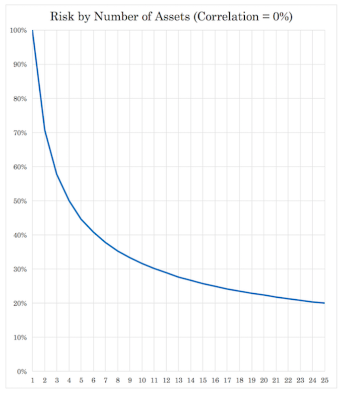
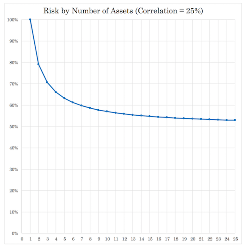
We can also see that once our correlation goes up to +0.25 among returns streams rather than +0.00, that the benefits of adding more returns streams is less and flattens out more quickly. And regardless of the extent of the diversification, the largest marginal benefits always come first.
Example
So, if you were to find 15 truly uncorrelated returns streams that each return three percent annualized at eight percent volatility, you’d still get the three percent, but would increase your reward to risk by a factor of about 4x. Or about 3 percent return at around 2 percent expected volatility.
If you needed a portfolio that yielded you 15 percent annually, you could borrow $4 for each $1 in equity depending on your arrangements. If the cash you borrow yields zero, you’d have a portfolio that give you expected 15 percent returns at 10 percent expected annualized volatility.
This isn’t bad considering that your menu is from a bunch of 3 percent returners with 8 percent volatility.
You added 5x (15 percent instead of three percent) the return but added only 0.25x (10 percent volatility instead of 8 percent) the risk.
This illustrates the positive impact of diversification when returns are truly uncorrelated.
However, finding what these sources of returns are is a different story.
You have traditional asset classes, stocks and bonds, which tend to be uncorrelated over long durations of time.
Then you have certain commodities, like gold, which can be good diversifiers when help in a small position in a portfolio (usually 5-10 percent allocation) that do a little bit better than cash over the long-run.
You have things like private investments – e.g., real estate, timberland, internet projects, reinsurance – that in some part act differently and can help build a better balanced portfolio.
But they don’t really fit the “liquid” part except for some reinsurance investments from that short list. They can provide income streams, but it can be hard to sell the investment itself.
Unlike a stock, which you can sell quickly from a computer or handheld device at whatever the current price is, real estate, websites, physical assets, and so on can take a lot longer. This is especially true if they are worth a lot (or you want a lot), as the pool of buyers thins out.
And you have certain liquid strategies that you can get from unique portfolio construction.
The volatility risk premium is one such source of returns that is uncorrelated with common asset classes.
How to create a liquid alternative
Anyone could create a liquid alternative. How could you make a liquid investment that is uncorrelated with market?
For example, creating a liquid alternative could be as simple as buying some stocks and shorting others randomly such that the beta cancels out and it’s more or less uncorrelated, or market neutral.
However, approaching the markets this way in terms of picking what’s going to be good and what’s going to be bad is difficult to do.
The range of unknowns is high relative to the range of knowns relative to what’s already embedded in the price of each security. The price of a stock or anything already reflects what’s known.
This makes your starting point such that almost everything is as equally good or as bad of a bet.
While it is not hard to know what companies will be good or bad in terms of future performance, it is hard to convert this knowledge into winning bets because these expectations are already part of the built-in consensus.
It’s not unlike sports betting. You have some teams that are much better than other teams. But it’s not easy to win these bets because you have a point spread to contend with along with the bookmaker’s keep priced in.
So, for even sophisticated traders, going long and short to be market neutral is hard to do well.
Randomly going long and short securities just to create a liquid alternative would be worse than useless.
Accordingly, construction is a key element to make them effective, such that they provide quality returns and quality risk-adjusted returns at low correlation to the broader markets and other asset classes.
Recommending the whole asset class doesn’t make a lot of sense given this important caveat.
While traders going long various stocks and stock indices don’t need to have picking skill per se – because stocks usually go up over time – with liquid alternatives how they’re engineered is very critical to how they perform.
Most hedge funds still commit the general error of being too correlated to traditional asset classes, often a +0.75 to +0.90 correlation (with +1.00 being perfect correlation) to their domestic equities markets.
Yet they still have very high fees even though their clients, in most cases, aren’t getting much of a differentiated investment product.
The choice to allocate to liquid alternatives
Liquid alternatives are not a hedge on risk assets.
If you are concerned about a drop in the stock market and you want to express this position, then the best way to do this is to express bearish positions on equities (e.g., short selling, owning put options).
Liquid alternatives are meant as a diversifier.
If you are trading or investing to begin with, then you’re doing so because you believe what you’re doing has a positive expected value/return and quality risk-adjusted returns.
A liquid alternative is a way to help diversify relative to the other things you’re doing as part of your overall investment strategy.
A low correlated alternative asset class can improve risk-adjusted returns in the same way an equities manager can improve their portfolio in that respect by adding in bonds. Just like a bond manager can build a better portfolio by adding in some equities.
The best case is when the liquid alternative in question has no correlation to what else you’re doing in your portfolio. However, it’s not strictly necessary for the correlation to be zero.
It should, however, have a positive expected return (i.e., will convey greater real spending power in the future) that doesn’t have much correlation such that it’s a differentiated return stream.
If you can do this, you’ll have a higher return for the same risk, the same risk with higher return, or some permutations thereof, or can improve on both.
Even for a trader or investment manager who can’t use leverage, or is constrained in terms of how much borrowed money can be used, you can still increase expected overall returns depending on asset allocation.
For instance, if you invest in a higher-returning alternative, you can reduce the risk of the entire portfolio while moving your allocation away from cash, bonds, and even stocks to get the expected return of the portfolio back up.
Construction of a liquid alternative
There are different ways to construct a liquid alternative.
One way is to find an investment that isn’t very correlated to traditional stock and bond investments.
For example, this might be something you do on your own that you personally manage. It could even mean a blog or social media channel you run and monetize in certain ways.
The income you derive from it is probably at least somewhat correlated with traditional investments. If companies are pulling back during down periods, that means things like advertising and referral partnerships might be pulling back as well, hurting certain types of private investments.
If you sell your own products and services, a rough patch probably means many consumers are pulling back on their spending as well.
But many things of that nature could be considered mostly uncorrelated, even if it’s not particularly liquid.
Things like timber, farmland, real estate, venture capital, and/or private equity are a source of alternative returns. They don’t have their prices marked to market daily so you don’t “see” your capital gains or losses in real-time.
And perhaps the illiquidity inherent in these types of investments are good in a way for managing the psychology behind the twists and turns of being marked to market constantly.
As a result, some things can ironically become more attractive to own just because you don’t have their prices constantly marked to market. But at the same time, it’s likely to overexaggerate the extent of your portfolio’s diversification.
But the purpose of this article is to focus more on liquid alternatives. So, while one’s view of illiquid alternatives could be positive, that’s not the current topic of conversation.
The main way of constructing a liquid alternative
The main method of constructing liquid alternatives is by going long some assets while shorting similar assets.
While some people choose to never short, if you don’t, you are missing out on a big way to help diversify your portfolio and help derive largely uncorrelated returns streams.
The long and short amounts are relatively comparable in order to hedge the relative market exposure to make them truly uncorrelated.
This needs to be accomplished in a way that assumes the longs will outperform the shorts.
This can be done in a way where a well-known characteristic of a company, commodity, bond, etc., is a good predictor of future performance, with something proprietary (e.g., based on data mining), or an improvement of something already known.
Example
As a popular example, it’s known that companies with low price-earnings (P/E) ratios historically outperform those with high price-earnings ratios over time.
Therefore, an example of a liquid alternative would be to go long the low P/E companies and short the high P/E ones.
This should be done in a way to equal the risk on each side.
While some take long/short strategies to mean equal dollar amounts on each side, this is often not the best tactic because the longs and shorts can have different risk and volatility characteristics.
It’s also often true with generalized diversification strategies. For example, the 60/40 and 50/50 portfolio pertain to weighting stocks at 50-60 percent and bonds at 40-50 percent in a portfolio.
The issue is that stocks are more volatile than bonds, so a 60/40 portfolio is really more like a 90/10 portfolio from a risk perspective (i.e., almost all the price risk is concentrated in stocks). And the 50/50 portfolio is really more so close to an 80/20 portfolio on the basis of risk.
In the case of a hypothetical long ‘low P/E’ portfolio and short ‘high P/E’ portfolio, the volatility of each side should roughly balance out.
High P/E stocks tend to be more volatile. They are more growth-like in nature as more of their cash flows are discounted out in the far future. This gives them a longer duration and therefore generally higher price sensitivity. (The concept of duration is most commonly applied to bonds, but is true with respect to virtually all investment assets in some way.)
Low P/E firms tend to be less volatile, earning more of their income in the near future and having shorter duration accordingly.
As a result, any trader looking to put on a liquid alternative of this type might want to put more (in monetary terms) into the ‘long low P/E’ portfolio and less into the ‘short high P/E’ portfolio based on the expected volatilities of each side.
For example, to get roughly risk with a stocks/bonds portfolio, a trader is likely going to want to be 30-35 percent stocks and 65-70 percent bonds to get them to even out.
There is also something to say for making such a portfolio not on the basis of stocks as a whole, but by sector. This way your weights won’t heavily long some sectors (which tend to disproportionately have lower P/E ratios) and short other sectors (which tend to have higher P/E ratios).
The general idea behind engineering liquid alternatives
By and large, the general idea is to go long the assets that are attractive in that particular measure and short the ones that are not, limiting market exposure to give it the ‘alternative’ characteristic.
If it has less correlation to the rest of your portfolio it will be diversifying and enhance returns in a risk-adjusted way.
If the stock market is comprised of two general types of stocks, X and Y, and if group X had some edge over group Y then you could have a position of X-Y to help diversify market exposure to X+Y.
Of course, this is an oversimplification, as X might outperform Y, yet X might be ‘higher beta’ than Y.
One way to create a type of alternative is to simply tilt a portfolio more toward X and less toward Y.
This is one to diversify a portfolio and with no short selling and/or (if desired) no leverage. This is a strategy for long-only investors or those who don’t want to get overly involved in their portfolios.
The downside is that a portfolio of X (overweighted) + Y (underweighted) will still have a relatively high correlation to the market, being weighted more toward some companies and away from others.
The benefits of an ‘X-Y’ (in whatever quantities of each) portfolio is largely in the ability to short and be uncorrelated to the broader market.
Trend following liquid alternatives
A trend following portfolio is another type of this general nature. The idea with a trend following portfolio is that as trends trend, it will sometimes be net long and sometimes net short.
Naturally it is correlated to the market at times.
But over longer time horizons, the net long and net short nature of it will ideally – if it’s a liquid alternative in the strictest sense – make it uncorrelated.
Strategic importance of liquid alternatives
Strategic diversification is more important than normal given the low future returns of traditional stock and bond investments.
Bond and stock returns over the past 50 years or so in the US has been a bit over 7 percent (US Treasury bond) and over 10 percent for stocks.
| Name | |||||||||||||||||||||||||||CAGR | ||||||||||Stdev | Best Year | Worst Year | Max. Drawdown | Sharpe Ratio |
|---|
| US Stock Market | 10.39% | 15.60% | 37.82% | -37.04% | -50.89% | 0.42 | ||
| 10-year Treasury | 7.21% | 8.03% | 39.57% | -10.17% | -15.76% | 0.34 | ||
| Cash | 4.69% | 1.01% | 15.29% | 0.03% | 0.00% | N/A |
In particular, because stocks are traditionally the ‘high return’ part of a portfolio, it is important for investors to find positive returns streams that are uncorrelated to standard equities investments.
Even small amounts of diversification matter.
The first small move toward diversifications has the largest marginal benefit. The benefit of adding ‘asset #2’ has a greater benefit than when adding ‘asset #3’ and so on.
It’s when adding no more new assets (‘correlated’) when the benefits stop accruing.
Correlations are also unstable.
Sometimes many assets that are usually uncorrelated or often go in opposite directions – e.g., the stocks and bonds relationship that most developed market investors have become accustomed to over the past several decades – but this changes over time.
Moreover, sometimes putting a certain amount of your portfolio in a certain asset might be ‘mathematically optimal’. (Gold at 5-10 percent of a portfolio, due its diversifying nature but lower returns, is a popular example.)
However, if investing whatever percentage of a certain asset is often too painful to endure when these returns streams don’t work or go against you, then that amount is too much.
And at times there will inevitably be periods where your portfolio doesn’t work the way you expect.
Risk-adjusted return expectations
The Sharpe ratio is the industry standard for assessing risk-adjusted performance. This is the ratio of excess return over cash divided by the volatility of a portfolio.
So, if your return on stocks is four percent and the return on cash is zero, and the volatility of stocks is 16 percent, then the Sharpe ratio is simply 4/16, or 0.25.
The ratio would be the same if stocks return 10 percent and cash returned 6 percent. You get the extra four percent either way.
The Sharpe ratio is far from perfect. For one, it treats all volatility equally.
‘Upside volatility’ is good. This is the type of volatility you want if you own a call option on a security.
‘Downside volatility’ is bad for those long assets (unless owning a put option).
The Sortino ratio attempts to correct for upside and downside volatility. As a result, well diversified portfolios tend to do better on the Sortino ratio than the Sharpe.
Moreover, the Sharpe ratio is made to fit the normal distribution, given it uses annualized volatility – which is typically measured using the assumption of normality.
Most investments are very much not normally distributed. The assumption of normality is used to simplify, even if it’s not particularly accurate.
An extreme example very non-normal returns is the use of options.
Buying an option gives you a little bit of downside, but a lot of potential upside.
Likewise, selling an option gives you relatively small positive returns, but every now and then you’ll receive a large (or very large) negative return.
The realized volatility of options is very lumpy given the large, but infrequent, bursts of high volatility and otherwise longer periods of volatility that you’re accustomed to.
Selling volatility often has longer periods of a higher Sharpe ratio and shorter periods where the ratio is very negative. A prime example of this was the volatility selling throughout 2017 before the February 2018 blowup.
Just like being long volatility tends to produce losses (known as theta decay) while once in a while it makes great returns.
Even despite all that, the Sharpe ratio can be very useful in comparing strategies so long as not applying it to strategies and processes involving highly non-normal distributions.
It is the most often referred to measure of risk-adjusted performance in investing circles when discussing investment strategies.
Accordingly, the Sharpe ratio is the standard metric to use even if it is imperfect.
The Sharpe ratio of the US stock market since the mid-1920s is just under 0.40. Since 1972, it’s been about the same (0.42), though aided since the 1980s by a large drop in interest rates.
If you stick with a 0.40 Sharpe ratio investment over the long-term, it will probably work out over the long-term, though nothing is ever certain.
A 0.40 Sharpe ratio means if you have an annualized volatility of 10 percent in your portfolio, you could expect to earn 4 percent per year annually over a long time horizon. Or, in basic terms, each 1 percent increase in volatility should expect you to get an extra 0.4 percent in annualized returns.
Sharpe ratios of 0.2-0.4 in asset classes is standard long-term.
When they get toward the lower end of that boundary, the risk isn’t commensurate with the expected reward. Conversely when they get toward the higher end of that range, the return relative to the risk attracts capital.
If you can create a portfolio with a 0.4 Sharpe ratio, and assuming normality in the distribution of returns – a better assumption the longer your time horizon – your chance of positive returns (relative to cash) on any given day is 51 percent.
(Since 1926, the number of positive days is actually 53 percent, but the Sharpe ratio since then is slightly higher than recent history and returns are not perfectly normally distributed. At the same time, we’re simply discussing a generic 0.40-ish Sharpe ratio strategy.)
For any given month, your probability of positive returns has been 56 percent. For a six-month period, its 61 percent. For any given year, it’s 67 percent. And for five and ten years, it’s 81 percent and 90 percent, respectively.
That sounds good, and it is. But that also means there’s a chance that you could hold a portfolio that emulates the stock market over ten years and not make any additional return over cash for a decade.
At the same time, finding a way to trade or invest that gives you as good of a return as the stock market – while not being correlated to it – would be a pretty good strategy.
Investment managers and traders typically try to get something better than that. Many strive for a Sharpe of 0.50 or better. Some aim for above 1.00 but that’s not easy to do, especially over longer durations.
But if you did manage to find a 0.40 Sharpe ratio strategy and it was uncorrelated with the stock market, the basic idea is you’d want to put as much in this strategy as you would the stock market.
Not that this is necessarily recommended. A big part of such a strategy, whatever it might be, is actively managing it.
If your strategy ‘recommends’ putting 10 percent in gold, but you can’t tolerate the volatility in gold such that that 10 percent would become a problem when it declines materially, then going up to only the amount you can stick with through a bad period is probably a better idea.
Liquid alternative strategies with risk-adjusted returns that emulate (or beat) the stock market are worth having and can improve a portfolio. It’s just a matter of keeping with them when they perform poorly, which will inevitably happen.
Three Sharpe ratio investment strategies?
Achieving very high Sharpe ratios, like 2.00 or above to throw out a number, are considered a type of ‘holy grail’.
They may appear to exist over short periods or in cases such as:
i) Volatility selling strategies may appear to get very high Sharpes over shorter benign periods, but eventually have deep drawdowns.
Vol selling is not necessarily bad on its own – see our write-up on the volatility risk premiums strategy.
But they are often presented as having high Sharpe ratios simply because nothing bad happened over that period.
ii) Strategies that have a type of first mover advantage, but don’t last once everyone else catches on. Anything that has profit potential will eventually attract competition.
iii) Strategies that have smaller capacities (e.g., proprietary data sets that can’t be deployed at scale).
iv) Illiquid strategies that don’t represent their risk accurately
v) Certain sustainable and high capacity Sharpe ratio strategies investment processes on their own.
With respect to the latter, they tend to fall into the second or third categories, where they have limited capacity (small and unique) or have some type of first-mover advantage that’s likely to eventually erode.
But even when they appear to be real, they are not enough to move the needle much for major institutional investors or large numbers of individual investors.
Many of these types of strategies tend to be more fleeting than legitimately good.
Telling good managers apart from bad managers is hard to do over shorter periods, unless they are really bad. (It may also be why some hedge funds last so long without providing anything that’s genuinely unique and of value-additive quality.)
The strategies tend to be smaller capacity, but not so incredible in reality. They also tend to be higher fee, which reduces their net return.
A hedge fund with a management fee of 5 percent and 40 percent performance fee – the ones pursuing these types of high Sharpe strategies – is taking a lot.
If they throw in the first 6 percent in annual returns for free, and the strategy achieves a 20 percent annual return, then a $1,000,000 investment would return:
– You get the first $60k thrown in
– The next $140k is subject to a 40 percent performance fee ($56k, leaving $84k net)
– Plus, a 5 percent management fee, which comes to $50k
– That comes to fees of $56k and $50k, or $106k total
– That 20 percent return (+$200k) is now just a 9.4 percent return (+$94k), or more than half taken up by fees
The Sharpe ratio is ultimately not as good of a measure as the total expected value (measured in monetary terms) provided to client portfolios.
On top of that, many of the sustainable “high Sharpe” strategies will tend to close themselves to new investment to retain an edge. They may even give their clients’ their money back eventually (once the owners of the fund have enough capital to deploy their strategies to capacity) to keep the returns of these strategies all for themselves.
Rather than high Sharpe strategies as a type of ‘holy grail’, modest return strategies that improve risk-adjusted returns (relative to a representative benchmark) while diversifying to the rest of your portfolio are underappreciated.
For an institutional investor, being able to employ the strategy at larger capacity is especially important to generate high management and performance fees.
Sticking with them through the bad times for good (but not insanely high) risk-adjusted returns is simply part and parcel of trading and investing.
If you have found a process or strategy that does provide a 0.50+ Sharpe long-term with low correlation to the rest of your portfolio, then that’s a great thing.
What to do when tough times come around for liquid alternative portfolios
Liquid alternative portfolios that are long/short in nature will go through inevitable dry spells or rough patches like all others.
When tough times hit your portfolio, the first question is why you believed in the process or strategy in the first place.
Basically, it boils down to what evidence or intuition convinced you to do these things in the first place.
When institutions engage in liquid alternative strategies they are typically doing so with respect to factors like:
…and so on.
Certain securities (like stocks underlying stably profitable firms over the opposite) will tend to outperform other stocks that don’t have these characteristics over the long-run.
Intuitively this makes sense as companies need to be profitable in order to validate any type of positive valuation. Companies that don’t make money aren’t worth anything.
These factors also show success beyond US stocks over a long time horizon and can also be applied to credit, commodities, currencies, interest rates (e.g., where to be on a yield curve).
Generally speaking, stocks with:
- good value
- positive momentum – fundamental (positive revenue and earnings trajectory) and technical (price)
- lower risk, and
- higher quality (profitability, margins)…
…are probably going to outperform those that don’t have these qualities over the long run.
A liquid alternative strategy might go long stocks and/or credit of companies that have the aforementioned qualities and go short – or underweight – those that don’t to obtain a largely uncorrelated returns stream to the market.
When this doesn’t work – the ‘bad’ is outperforming the ‘good’ – then you don’t want to all of a sudden prefer the bad securities over the good.
(This of course assumes the work to select these quality stocks is being done well.)
What do the numbers say?
During a rough patch in any strategy, ask whether the recent rough patch is surprising or within the distribution of expectations.
Sometimes these shocks occur due to a liquidity dislocation that has no relevance to the general quality of the security selection itself – other than that they’re nonetheless susceptible to them.
All financial assets can sell off, even temporarily, due to a financial crisis, bank panic, natural disaster, asset bubbles, and other events.
If you are using strategies that have worked over the long term with plenty of historical data to back them up, then a painful but not historically bad period of performance shouldn’t change your views on what to do going forward.
If you believed in something before a bad quarter or bad year, it doesn’t make sense to change your view just because of a tough period.
The biggest mistake in trading and investing is almost implicit in the idea of changing up what you do. It’s not whether the past 6 to 12 months have been like but rather whether your judgment is sound or not.
What if a strategy has been poor over longer time horizons?
This is not the case for multi-factor quantitative stock selection.
However, it can be somewhat true for some individual factors, such as value (for equities) and trend for markets in general. (Markets tend to operate in trends, but predicting when they switch is hard to do.)
Since the 2008 financial crisis, value has done particularly poorly relative to other types of stocks. The post-financial crisis peak for value occurred in April 2010. It has underperformed by nearly two standard deviations since then relative to the total period running from 1926 to the present.
Though that’s not ideal, a statistician wouldn’t necessarily worry.
The graph below shows cumulative and 10-year rolling returns of the Fama French HML strategy from 1926 to the late 2018.
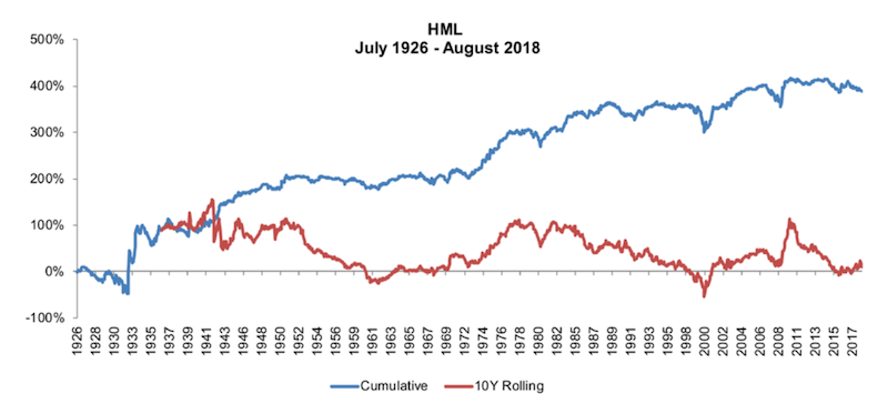
(Note: This portfolio is derived from going long high book to market and short low book to market. This is essentially going long the companies with quality value and shorting those with poorer value.)
Value had exceptional periods in the mid-30s as well as from the early-70s to late-80s. It’s been roughly flat since the mid-00s.
At the same time, 400+ percent cumulative return (5x) over nearly 100 years isn’t terrible for an uncorrelated long/short strategy.
There are long periods where it’s flat for years and periods where the cumulative 10-year return is about 100 percent. Ten-year cumulative negative-return periods are rare.
It’s not something you’d want a large amount of your portfolio in, but having some allocation to it could be reasonable.
During these times, when a strategy is down, you must understand what’s going on and make a judgment, ideally as rationally and quantitatively as possible, though not necessarily purely so.
Realized recent returns will not tell you a whole lot.
Two standard deviation events are not simply things to dismiss entirely. It’s important to know whether the world has changed and a strategy that was formerly a good idea is now a bad one.
Intuition is important. Are profitable, high-margin companies better than their opposites? This will always be true.
Other factors to consider
One possibility is that too many people now follow certain strategies, eroding their advantage.
When many people pursue a strategy, any margins to be had pursuing it become smaller.
Accordingly, many investors try to understand the relative cheapness or expensiveness of a factor on its own.
Some investors have their own metrics to measure this, such as a ‘value score’.
What is the value score of the securities the factor likes relative to the value score of the securities it dislikes.
For the value factor, the value spread (value score of ‘liked securities’ minus value score of ‘disliked securities’ will by definition be positive between the securities it deems cheap relative to those it deems expensive.
If the value factor were to get arbitraged away – or more money chasing the same types of trades – then the value spread should tighten. Spreads for other factors (e.g., momentum, carry, size, etc.) would likewise tighten.
If value was getting arbitraged away, we would have expected the value factor to see better than average returns since the 2008 financial crisis followed by a period of relatively sparse returns – or worse depending on how far it went. But that didn’t occur.
Generally, if a strategy catches on and other people copy it, then you should expect large profits at first – even a bubble (like everyone chasing tech from 1998-00), followed by sparse returns following.
It could be that the transaction costs involved in trading these factors could be higher, eating into returns in a different way. But there’s also no evidence to support this. Value stocks are not underperforming because they’ve become more expensive to trade.
It could also be that there’s an issue with how value is measured.
Value is generally determined by projecting a company’s future cash flows and discounting them back to the present at an expected rate of return (example with respect to Apple stock).
Then comparing that price range (derived from the discounted cash flow analysis) to its current price in the open market. If the price based on the discounted cash flow analysis is lower than the market price, then an investor might deem the security cheap, or having a high value score if participating in fundamental factor investing.
Value can also be measured using standard multiple measurement, such as price/earnings (P/E), price to book (P/B), EV/EBITDA, and so on.
P/B – more traditionally book to price – is one of the most popular measures of value that goes back more than 100 years and has been used to construct some of the most popular value indices (e.g., the work of Fama and French).
Doing this industry by industry can help mitigate any distortion in what the factor deems ‘cheap’ and ‘expensive’.
Technology companies tend to have low book value relative to a capital-intensive, asset-heavy industry like manufacturing or banks (where banks use capital to make money).
But this is because their business models are different and tend to be more about data than physical assets or money/capital. This makes their book values small relative to their prices.
Without going industry by industry, a trader looking to create a liquid alternative by going long the low P/B securities while shorting the high P/B securities might end up long a lot of banks, oil and gas firms, REITs and other finance companies and short a lot of tech.
Isolating the factor industry by industry is likely to do a better job to avoid being lopsided on the sectoral allocation.
Value wins on average over the long term. Theoretically it should, given the fundamental value of a business relates to its ability to generate cash, and that a higher cash yield relative to its present value (i.e., its price) should provide superior positive returns.
However, it can underperform severely even over the course of about a decade.
But it’s unlikely value is bad because of the three potential issues outlined:
- i) value spreads have closed (no evidence)
- ii) transaction costs are higher (no evidence)
- iii) traditional value measures are outdated relative to today (unlikely)
And if a factor is ‘broken’ – or it doesn’t measure what it’s supposed to, or is measured inaccurately or not very precisely – this is likely to generate random returns, not systematic losses.
In the end, if a strategy is not working to expectation, then you need to evaluate why you believe it should work in the first place. It should be backed by evidence and also economic intuition.
Keeping an open mind is important. Looking to the past to inform the future is only so good as the past being a good representation of the future. Big changes can occur to markets that can make hundreds of years of evidence irrelevant, so it’s important to know the cause-effect relationships.
As for value, there hasn’t been a material structural break in relative value or how it’s generally measured – especially for companies within the same industry.
Ultimately, one should change their mind based on evidence, large enough numbers to change the historical evidence, or something supported by observation.
None of these necessarily apply to the value factor today, or why being long the ‘value spread’ shouldn’t necessarily be a quality liquid alternative if constructed well.
Liquid alts as the stock-bond correlation becomes less reliable
The role of bonds as a hedge to stocks has been a popular investing canon.
From the early-1980s to early-2020s, stocks and bonds mostly moved inversely to each other.
Inflation was low and steady, so changes in growth were the main driver, leaving stocks and bonds to be good diversifiers to each other (stocks doing better in a high-growth environment, with bonds doing better in a low-growth environment).
When those markets fall together, traders and investors tend to look for other, sometimes riskier, forms of protection.
In 2021-2022, when the negative stock-bond correlation broke down most significantly with wide discounted inflation outcomes, money piled into liquid alternative mutual funds and ETFs, posting $60 billion in inflows in 18 months.
Sometimes called hedge funds for the masses, liquid alternative funds allow individual investors to diversify their portfolios using more complex hedge fund strategies, including everything from options to convertible bond arbitrage.
Roughly $200 billion currently sits in such liquid alt funds, according to Morningstar Direct.
The funds lack some of the protection offered by hedge funds, which usually require investors to lock up their funds, thereby allowing withdrawals only at specific intervals (e.g., being able to withdraw one-eighth of one’s investment per quarter).
That prevents hedge funds from being forced to sell positions in order to meet investor redemptions, which could hurt performance for remaining investors given selling’s effect on market prices. No such protection exists for liquid alts.
Performance among liquid alts can vary widely, as there is no uniformity in strategy – outside of being liquid and uncorrelated to traditional asset classes.
Moreover, they carry hefty fees of anywhere from 0.5 to 3 percent, potentially deterring investors who have grown accustomed to getting more traditional products that charge less than 0.1 percent, like standard stock ETF funds that passively track an index.
Some of the best-performing categories among liquid alts in 2022 – when stock and bond indexes did poorly – were systematic trend strategies that follow price-momentum by trading futures, options, and swaps.
Conclusion
Liquid alternatives are an asset class that involves providing return streams that are liquid (unlike many alternative investments) and largely diversified and uncorrelated to other major asset classes.
Many liquid alternative strategies involving going long assets or securities that are expected to provide a positive spread on a certain variable while shorting those that do the opposite.
This can be as basic as going long industrial stocks with low price-to-book values against industrial stocks with high price-to-book values. This is a play on the ‘value’ factor.
It may even involve proprietary data mined using ample computing power.
It can be done for any asset class, including equities, credit, currencies, commodities, and even interest rates.
Long-only investors or those who don’t or can’t use leverage can also take advantage of some liquid alternative processes by tilting their portfolios toward the ‘good stuff’ and away from the ‘bad stuff’ to improve expected returns outcomes.
Any strategy should nonetheless be based on evidence (such as backtesting over a long time horizon, including recessions and other market dislocations) and sound economic reasoning and intuition.