Market Neutral Strategy with Covered Calls and Puts


A market neutral strategy involves selecting individual securities to buy and short-sell such that roughly equal amounts of money are both long and short the asset class.
The market neutral strategy is typically applied to equities, given the vast selection to choose from. Though it can also pertain to other asset classed like fixed income and commodities.
One can be “neutral” on commodities but be long and short various types of them. Going long and short fixed income can be similar to security selection in equities or it can be used to express views on the future shape of the yield curve, for example.
In this article, we’re going to introduce a simple strategy that involves being market neutral but with the twist of being overlaid with options.
Market Neutral Strategy with Covered Calls and Puts
We’re going to set up an example portfolio where we’re short “the market” as represented by the exchange-traded fund SPY. As a popular legacy ETF with decades of history, it is widely traded and has a large and deep options market.
To be market neutral, we select a handful of stocks to go long to roughly offset the amount that we’re short. These can be of our own choosing, or they could even match the index itself to have a perfect hedge. (Without an algorithmic program, this would be extraordinarily tedious.)
Let’s say we go long three stocks:
– Twitter (TWTR)
– Altria (MO)
– ExxonMobil (XOM)
If we’re short 100 shares of SPY, that means to put a roughly equal amount of money on the other side, we’ll have to buy about 300 shares of the other stocks.
We buy in increments of 100 because we’ll be overlaying options on these stocks, as options have 100 shares per contract.
So our entire trade becomes:
– Short | 100 x SPY
– Long | 300 x Twitter (TWTR)
– Long | 300 x Altria (MO)
– Long | 300 x ExxonMobil (XOM)
Behind the Idea of Options Overlay
In the options market, traders make a prediction about how much a stock will move between the current price point and expiration of the options contract. This is called implied volatility.
Implied volatility (IV) is a bit different from what’s known as realized volatility (RV), or the type of volatility that plays out in practice. The profit is the difference between the two.
Over long periods, markets do a relatively decent job of predicting future volatility.
But implied volatility is typically higher than realized volatility. This is done on purpose.
In options trading, especially when you sell options, when you are wrong it is very costly or even lethal.
While options and derivatives were originally designed to help hedge risk, some have naturally used them to speculative on securities in a leveraged way. It can be psychologically enticing to have a bias toward selling options given the premiums at stake, but nonetheless bad if these options fall sufficiently in-the-money (ITM).
Selling options (sometimes called being short gamma) involves being entitled to a certain premium that the buyer of the option pays you. That effectively means the option seller is insuring against that risk and has to pay out, in the amount entitled to the buyer, should the option go ITM.
When options do go ITM, this often means the seller is on the hook for multiples of the initial premium.
Because of this, options sellers effectively charge a premium to compensate them for this risk.
This provides some type of what you could consider a type of risk premium (i.e., a volatility risk premium).
When plotting out Apple (AAPL) stock through the first ten months of 2018, you can find that implied volatility was on average higher than realized volatility with a lot of fluctuation in between.
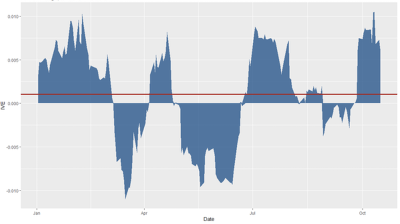
In other words, when IV is greater than RV, this provides an advantage to options sellers on aggregate. This helps compensate for the outsized loss or “risk of ruin” potential associated with selling options.
Based on the diagram, there is far more profit to be had in trying to get the swings correct. But this is very difficult to do and is why most people lose money trading options.
On the other hand, a trader who was short volatility on Apple but covered their position would have made a profit if executed in a meticulous way.
Options Overlay
In each of our trades, we are going to cover the position with an at-the-money (ATM) option, or the closest approximation to what an ATM option would represent given the current price of the underlying security.
We’re also going with shorter duration trades. On each of these tickers, weekly options are available.
That means for our short position (i.e., SPY), we would enter an ATM put.
For our long positions (i.e., TWTR, MO, XOM), we enter ATM calls.
These are known as covered puts and covered calls, respectively.
When you cover a position by owning or shorting the underlying stocks (with calls and puts, respectively), you take away the unlimited downside risk associated with selling options.
The premium associated with short-term options
Short-term options tend to have this premium embedded in them.
Let’s first consider the short side of the trade in terms of SPY.
SPY
For example, consider the case of a weekly SPY ATM put option (technically $0.26 per share OTM) trading at $3.75 per share.
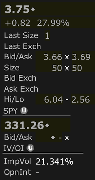
(Source: Interactive Brokers internal interface)
With 100 shares per contracts, that’s $375. The price of SPY is $331.26. One hundred shares comes to $33,126.
If we take the price of the contract and divide by the market value of the shares, we get:
Payout percentage = $375 / $33,126 = 1.13 percent
If these shares go ITM – which would close out our entire position after expiration – we could add those $0.26 per share to the total ($26 per contract).
This would increase the payout percentage to 1.21 percent. That $26 added to the $375 gives a potential return of up to $401.
That 1.2 percent seems like a large payout for a weekly option. And it is.
If we annualize that amount – 252 trading days per year divided by 5, or about 50 weeks effectively (holidays lower the number of trading days) – this comes to:
Payout annualized = (1 + 0.012)^50 – 1 = 81.6 percent
If we do simple multiplication, or 50 weeks multiplied by 1.2 percent per week, then it’s 60 percent.
Stocks don’t typically move up or down 60 or more percent per year, especially an index, where the collection of securities normally smoothes out its volatility relative to most individual securities or sectors.
But that 60 or ~80 percent isn’t what we’ll actually get because some of the time the stock will be OTM. When this is the case, we’ll not get the full premium as the total profit on the trade depending on the amount of capital losses.
Sometimes the capital losses will swamp the premium (and it can be by a lot) and this will produce a loss for this leg of the trade altogether.
So, we need an estimation of how often this is going to be the case and reasonable estimates of the loss to make an approximation.
We can see from the following set of metrics on the US stock market over nearly five decades that the number of positive periods for the US stock market (number of months in which it goes up) is about 63 percent. That’s also true for the weekly level.
| Metric | | | | | | | | | US Stocks (August 1972 to September 2020) |
|---|
| Arithmetic Mean (monthly) | 0.94% |
|---|---|
| Arithmetic Mean (annualized) | 11.85% |
| Geometric Mean (monthly) | 0.84% |
| Geometric Mean (annualized) | 10.49% |
| Volatility (monthly) | 4.50% |
| Volatility (annualized) | 15.60% |
| Downside Deviation (monthly) | 2.93% |
| Max. Drawdown | -50.89% |
| US Market Correlation | 1.00 |
| Beta(*) | 1.00 |
| Alpha (annualized) | 0.00% |
| R2 | 100.00% |
| Sharpe Ratio | 0.42 |
| Sortino Ratio | 0.61 |
| Treynor Ratio (%) | 6.64 |
| Calmar Ratio | 0.66 |
| Active Return | 0.00% |
| Tracking Error | 0.00% |
| Information Ratio | N/A |
| Skewness | -0.56 |
| Excess Kurtosis | 2.14 |
| Historical Value-at-Risk (5%) | -7.12% |
| Analytical Value-at-Risk (5%) | -6.47% |
| Conditional Value-at-Risk (5%) | -10.13% |
| Upside Capture Ratio (%) | 100.00 |
| Downside Capture Ratio (%) | 100.00 |
| Safe Withdrawal Rate | 4.33% |
| Perpetual Withdrawal Rate | 6.09% |
| Positive Periods | 366 out of 584 (62.67%) |
| Gain/Loss Ratio | 1.02 |
| * US stock market is used as the benchmark for calculations. Value-at-risk metrics are based on monthly values. | |
So, if we figure that we have about 50 weekly options to play per year and 63 percent of those periods are positive, put options will go ITM about 37 percent of the time.
This comes to being ITM about 18 times and OTM about 32 times.
And let’s assume that we get that 1.2 percent per week each time, and of the 32 times it goes OTM, we lose 1 percent (i.e., the stock market declines 2.2 percent – 1.2 percent minus 2.2 percent = 1.0 percent).
During the 18 expected times it goes down, it doesn’t matter how much it declines as the covered put caps the upside.
Expected value = 0.012 * 50 – 32 * 0.01 = 28 percent
Is this a good assumption? It’s hard to say, though it seems reasonable on the surface.
The risk with any covered strategy is that the underlying security goes against you by quite a bit and you end up losing money in excess of the options premium.
Now let’s consider the long side of the trade.
TWTR, MO, XOM
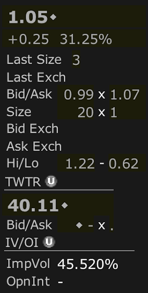
Twitter (TWTR)
Twitter’s ATM weekly call costs $1.05 per share or $105 per contract (per 100 shares).
Since the shares are $40.11, it’s already slightly ITM, but it’s the nearest expiry. When figuring the weekly potential return we’ll have to subtract this out.
The return on this comes to:
Potential Return = (1.05 – 0.11) / 40.11 = 2.3 percent
Our breakeven point would be the premium minus the strike price, or 40.00 minus 1.05, which is 38.95.
It’s also relevant to note that when something is already ITM it increases the probability that one will receive the maximum return. When something is OTM it decreases the odds.
Altria (MO)
For Altria, the ATM weekly calls costs $53 per contract.
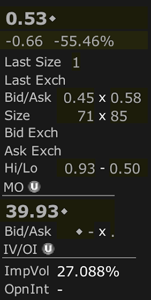
Shares are $39.93, so they are $0.07 per share OTM. The potential return is equal to:
Potential Return = (0.53 + 0.07) / 40.00 = 1.5 percent
The breakeven point is the current stock price (since it’s below the strike price) minus the options premium, or 39.93 minus 0.53, which comes to 39.40.
Altria’s earnings tend to be more steady over time as a consumer staple relative to Twitter, whose earnings are positive but small and relatively unknown over a longer time horizon.
ExxonMobil (XOM)
ExxonMobil’s weekly ATM call comes to $82 per contract.
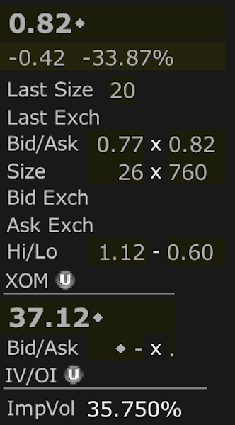
The stock is at $37.12 per share, leaving it $0.12 ITM. The potential return thus equals:
Potential Return = (0.82 – 0.12) / 37.12 = 1.9 percent
Total potential returns
To roughly equal the SPY short, we own 300 shares of each individual stock and therefore sell 3 covered calls on each.
If we sum up our potential returns – 0.94*3 + 0.60*3 + 0.70*3 – that comes to $6.72. With 100 shares per contract, that’s $672 for the week.
Adding the $401 from the short SPY side of the trade, that’s $1,073.
One can adjust those example figures up if more account equity is available to dedicate to such a strategy, though past a point putting anything on at significant scale is difficult.
What can go wrong?
The probability is low that all trades will land ITM and you’ll receive the maximum return. Markets move. Each security will find a new equilibrium point at the end of the week.
If they move enough in a direction against you, you will lose money. That’s all part of the game. It will happen often. Selling volatility during 2008 would have produced major losses in a variety of ways.
For example, let’s say equities go up that week. So, all of your individual stocks go ITM. That likely means that the short SPY trade may have produced a loss.
You have a 1.2 percent “buffer” before that individual trade produces a loss. For the entire trade structure to produce a loss, there would need to be at least $1,073 worth of losses somewhere.
If that came from SPY, that would mean a 3.2 percent up move ($1,073 total premium divided by $33,065 notional share value).
Or it could mean something like an 8.9 percent loss on Twitter ($1,073 / ($4,011*3)), or around a 3 percent loss on each individual stock.
It’s also not out of the question that all of the trades produce a loss. While being market neutral in theory sounds good because you’re reducing your overall beta there is idiosyncratic risk to deal with.
For instance, Ford and General Motors are similar companies. But being long Ford and short GM doesn’t guarantee any type of hedge.
In theory they should act in that manner as automotive stocks. But they can diverge in different directions for reasons specific to each business or factors related to the underlying markets for their securities.
The SPY could go up while the stocks you pick could go down. The way to hedge against this is by modeling the stocks you select on the SPY to perfectly hedge, though, as mentioned above, this is impractical for smaller trading operations).
Selling covered calls and puts is fundamentally a short volatility trade.
It relies to an extent on markets holding themselves together. A decent amount of the time they don’t do that, so caution must be heeded when exploring adding any type of volatility risk premium strategy to a portfolio.
Final Thoughts
A market neutral strategy is fundamentally about neutralizing one’s beta (or correlation) to a particular market. This is hard to do in terms of picking winners and losers.
One market neutral strategy involves covering each side of the trade with call options (on long trades) and put options (on short trades).
Then the trade goes from less about picking what’s going to perform well and perform poorly, to betting more on volatility.
Volatility tends to be “overpriced” in the markets because it’s essentially a type of risk premium. In other words, realized volatility tends to be lower than implied volatility.
It’s a form of compensation that traders earn for providing protection against unexpected market volatility, similar to underwriting and providing insurance.
We can bear this out when looking at options prices and annualizing options-related returns related to the price of a stock.
For example, the weekly volatility of a consumer staple stock like Johnson & Johnson (JNJ) comes to 80bps (0.80 percent), which is 49 percent annualized taking 252 trading days per year (5 days per typical trading week).
For AT&T, another relatively calm dividend stock, this annualized figure comes to 51 percent.
Volatility must be structurally overpriced to incentivize options sellers to enter the engagement, given the potential risk of loss is so large on a standalone basis.
However, volatility is not necessarily overpriced by a large amount and not perpetually overpriced.
As the Apple (AAPL) volatility graph showed above, there is a lot of variation where realized volatility does indeed run above implied volatility.
Selling volatility is generally one of those strategies that produces winners with fixed upside for a certain amount of time and is punctuated by large, sharp losses.
Covered calls are structurally similar to a short put. It has the same payoff structure of limited upside but a lot of downside (the stock going to $0 in the case of equities, while interest rates and some commodities can go below zero).
There are times when this strategy will make money and lose money like all others.