How to Build A Commodities Portfolio


Commodities are often overlooked in portfolios and tend to get more attention when other asset classes perform less well.
But commodities have value in a portfolio as alternative returns streams, a source of hedging (e.g., some price pressures in an economy are due to commodity inputs), currency alternatives, and entities that are subject to their own supply and demand characteristics.
We’ll look through at how to build a commodities portfolio in this article.
Key Takeaways – How to Build A Commodities Portfolio
- Start with a small strategic sleeve: in most diversified portfolios, 2%-10% commodities is realistic.
- It’s enough to improve diversification and inflation protection without dominating risk.
- You can think of exposures like gold separately, as it functions more like a currency than a traditional commodity.
- Treat commodities as a risk diversifier, not an income asset: they can hedge inflation surprises, add alternative return streams, and respond to supply and demand more than corporate earnings.
- Avoid naive index exposure: many passive commodity indices are energy heavy, can suffer roll costs, and may give you unstable volatility.
- Build a better allocation by risk balancing across sectors.
- Reduce energy concentration and spread exposure across energy, grains, industrial metals, precious metals, softs, and livestock.
- Add modest active tilts (optional).
- Emphasize carry or roll yield, trend, and fundamental signals while keeping sector limits to prevent concentration.
Overview
Commodities are nowhere near as popular as stocks and bonds as an asset class.
Pension funds largely concentrate their holdings in stocks, bonds, and other forms of equity like real estate and alternatives.
Retail traders and investors have very little exposure to commodities.
The main players in commodities are those who need to physically transact in the space.
To a lesser extent, there are global macro hedge funds, CTAs, and dedicated commodity traders.
The inflationary 1970s saw a pickup in commodities trading as stocks and bonds struggled to keep pace, losing value in real (inflation-adjusted) terms.
However, once inflation was reined in through a large increase in real yields in the early 1980s, commodities fell, and stocks and bonds embarked on a new 20-year bull market.
Stocks vs. Yields (1980 to 2000)
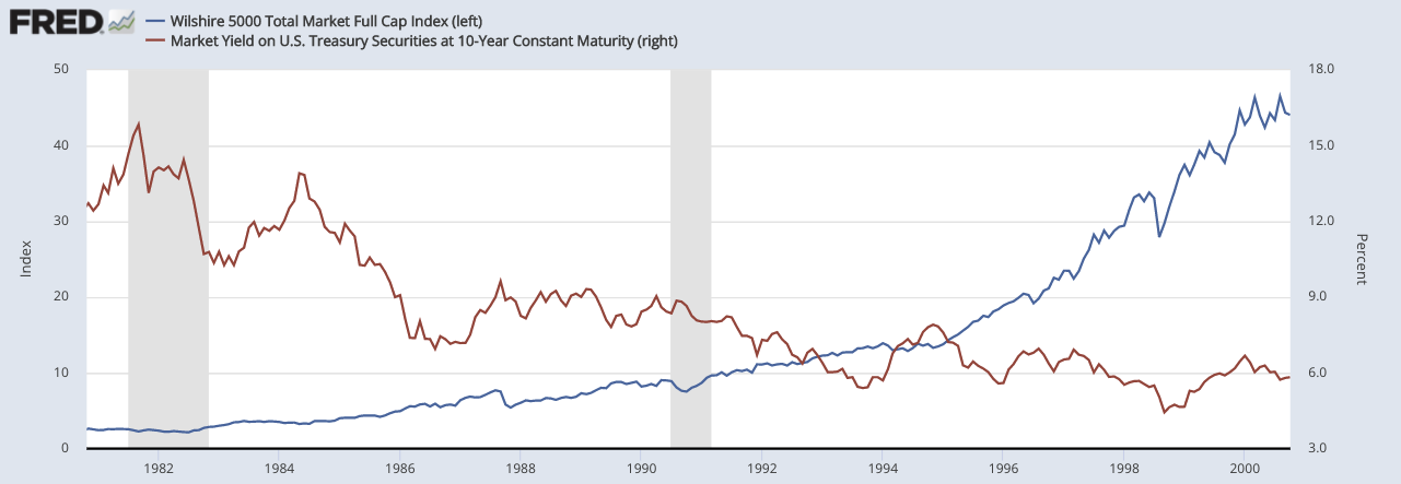
(Sources: Wilshire; Board of Governors)
As an asset class, commodities gained in popularity again during the 2000s, but experienced poor performance in the 2010s as inflation stayed low and many commodity prices fell due to oversupply.
Now, in the 2020s, public interest in the asset class is rising again.
Commodities have tended to be good diversifiers during periods of rising inflation or when inflation and inflation expectations are volatile.
How commodities are typically added to a portfolio
During the 2000s, commodities trading and investing was dominated by passive portfolios that were tracking indices.
These include the S&P GSC Index and the Bloomberg Commodities (BCOM) Index.
GSG is a popular ETF that was formed in 2007.
But recently traders and other market participants have become more aware of the flaws in these approaches.
These include:
- unfavorable contract roll costs
- poor sector diversification (e.g., too much energy), and
- missed active opportunities
What does a “good” commodities portfolio look like?
In this article, we look at the benefits of commodities as an overall asset class, and then take a look at the potential to better a commodities portfolio over a passive approach.
This can mean:
- better balancing of risk across commodity sectors
- risk management in commodities
- active tilts over passive indices based on strategies that have been compensated with better returns historically
For a long time, traders and investors have sought out alternative asset classes to diversify stock and bond portfolios that are dominated by equity risk.
For example, a 60/40 portfolio, which is quite typical of pension funds, has about 60 percent stocks and 40 percent bonds.
Even though it’s sort of balanced by money weightings, it’s not balanced by risk weightings.
Since stocks are typically 2x to 3x more volatile than bonds (depending on what types of stocks and bonds), that allocation is actually more like an 85/15 or 90/10 mix in terms of risk.
How to balance portfolios better
A balanced portfolio is designed to more efficiently capture the upside relative to the downside.
Another way to put it is improving reward relative to risk – i.e., getting more return per unit of risk.
Commodities are one thing to include in addition to fixed income and equity allocations.
Commodities’ popularity has varied through time. Many believe since commodities don’t produce income, they have no long-term use in a portfolio.
However, this perspective misses the potential for the diversification impact of their returns streams.
If adding something to a portfolio reduces your risk more than it reduces your return, you can work off that ratio.
For example, if a portfolio has 10 percent volatility and 5 percent expected return (0.5x return to risk ratio), and adding something reduces the volatility to 9 percent and return to 4.8 expected percent (0.53x return to risk ratio), if you return the portfolio’s volatility back to 10 percent, then you can get 5.3 percent expected return, an improvement of 30bps.
Volatility in a portfolio is like a dial. It can be adjusted up or down through leverage or leverage-like techniques (when wanting more return) or by holding cash against volatile assets (like crypto or long-duration/highly leveraged stocks) to make them less risky.
Improving return relative to risk is commonly called risk-adjusted returns.
We’ve written on the idea of balancing portfolios better in other articles.
- The Math Behind Portfolio Diversification
- How to Balance Risk to Achieve More Return Per Each Unit of Risk
- Building a Balanced Portfolio with Options
- Building a Balanced Portfolio with VRP Overlay
Investor pushback against commodity allocations
Over the long term – a multi-decade horizon – commodity returns have been diversifying.
However, many commodity indices suffered large drawdowns during the 2008 financial crisis, with little recovery in their prices during the disinflationary 2010s that followed.
Some market participants have accordingly questioned whether there is a positive premium in commodities.
Others have ethical concerns or sustainability or ESG-related reasons for staying out of commodities.
Yet inflation has let many traders know that adverse shocks in that variable can hit stocks and bonds alike.
Stocks and bonds are not inherently diversifying in inflationary environments because higher interest rates hit their prices due to how their cash flows are discounted.
The reality is that most portfolios are exposed to rising inflation. And commodities are one of the only types of assets to have provided reliable inflation protection as well as positive long term returns.
In the past, the majority of commodities have tracked passive indices.
These include ones like the S&P GSCI (GSCI) and the Bloomberg Commodity Index (BCOM).
While these indices do provide exposure to a broad set of commodities, their allocation is largely based on production quantities or market liquidity.
What this means is that there’s a concentration of risk in sectors that dominate global production, such as energy.
And energy has tended to correlate with risk assets more often than not (though not always).
But other commodity sectors have shown low correlations to each another.
Accordingly, a portfolio that balances risk across commodity sectors can better diversify idiosyncratic risks and therefore deliver better risk-adjusted returns.
In addition, passive indices have historically shown large swings in realized volatility, especially during periods of drawdown or in cases of geopolitical conflict (e.g., 1991 Gulf War, 2022 Russian invasion of Ukraine).
This presents a position sizing challenge to traders.
This can be mitigated by dynamically adjusting position sizes to better help target a more stable amount of portfolio volatility.
And commodities portfolios can be improved through active tilts based on factors such as:
- supply-and-demand fundamentals
- roll yield
- global macroeconomic data, and
- price trends within the commodities sector
With all of these features – risk balance across different commodities and commodity groups, risk targeting, and active tilts – traders, investors, and other market participants can make significant improvements to their commodity portfolios.
Benefits of Commodities in a Portfolio
An allocation to commodities offers traders and investors three main potential benefits:
- positive long-term returns
- low long-run correlations to stocks and bonds, and
- a hedge against inflation
Below we take a look at some of the theoretical and empirical evidence supporting each of these.
Commodities as a source of long-term returns in a portfolio
An investment in commodity futures has historically provided significant positive returns.
The chart below takes into account a very long data set comparing the returns to a portfolio of commodites futures to investments in global stocks and government bonds over nearly 150 years.
All three (stocks, bonds, commodities) have generated comparable positive risk-adjusted returns.
And because commodities have shown low correlations to equities and government bonds on average, a portfolio made up of all three has provided better risk-adjusted returns than a standard 60/40 portfolio of only stocks and bonds.
Commodities over the Long Run
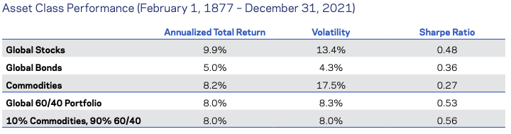
(Sources: Chicago Board of Trade, Commodity Systems Inc., S&P, Goldman Sachs, Bloomberg, and DataStream.)
(Commodities is a hypothetical equal-weighted portfolio, which takes equal notional weights of all commodities in the basket at each point in time. The risk free rate used to calculate the Sharpe ratios is New York call money rates until 1889, the New York Times money rates until 1918, secondary market rates on the shortest term U.S.bonds available until 1931 and T-bills thereafter. A rolling one-year average of the short- term rate is used. Aggregate global stocks returns are represented by GDP-weighted G6 (US, UK, Germany, Japan, Canada, and Australia) equities. Global bond returns are represented by GDP-weighted G6 government bonds. Global 60/40 is based on a 60 percent Global Stocks and 40 percent Global Bonds.)
__
The idea of going long commodity futures has had a theoretical since at least the days of John Maynard Keynes in the 1920s and 1930s.
The 1930s saw a big drawdown in stocks due to the Great Depression and a run-up in commodity prices, leading to shifts in thinking on the asset class similar to the 1970s and 2020s.
Commodity producers usually have concentrated businesses that are reliant on only one or two products, crops, metals, fertilizers, and so on.
To mitigate their price risk, they hedge by short-selling commodity futures. This creates a premium for investors who go long.
In other words, those who hedge are willing to pay an insurance premium as a way to stabilize future revenues.
In turn, this premium can be earned by traders and investors who are willing to bear price risk. (This occurs in all asset markets where derivatives and options exist.)
The long-term premium is likely to exist in the form of commodities’ exposure to economic growth.
While individual commodities’ macroeconomic exposures – e.g., to growth, inflation, interest rates – vary widely, a portfolio of commodities will tend to show some positive sensitivity to growth.
When economic times are good, this creates more demand for energy, base metals that feed into industrial processes, and other commodities that are used to create more goods.
Commodities as a source of diversification
Commodity prices are also influenced by fundamental supply-and-demand dynamics, commodity returns have historically shown a fairly correlation to other asset classes, as shown below in the next chart.
Nonetheless, there is a lot of variation in this correlation.
Traditionally, traders and investors have thought of commodities as being a “pro growth” asset class and therefore correlated positively with equities.
However, inflation typically negatively hits stocks when it means that interest rates will rise faster than what’s discounted, causing a fall in their present values due to the inherent process by which their future cash flows are discounted.
Other inflation protection assets and “alternative investments” have shown much higher average correlations to stocks or bonds.
This includes private equity, real estate, commodity-/natural resources-focused stocks, and inflation-linked bonds.
Private equity and real estate are both forms of equity. And inflation-linked bonds carry a correlation to their nominal counterparts because they’re both impacted by the interest rate component.
Chart B below shows that during periods of greater inflation volatility and “uncertainty” (defined here by the relative size of growth and inflation surprises), stocks and bonds have not done as well diversifying each other (because they tend to positively correlate during inflationary periods or when inflation volatility is larger than growth volatility), while commodities have been better diversifying to both.
Low Correlations to Major Asset Classes, Especially Amid Inflation Uncertainty
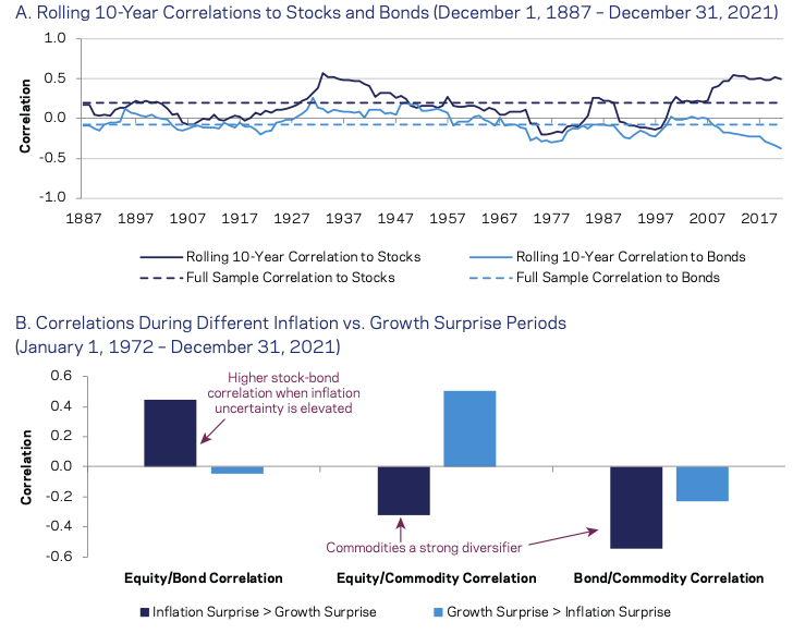
(Sources: Chicago Board of Trade, Commodity Systems Inc., S&P, Goldman Sachs, Survey of Professional Forecasters, Bloomberg, DataStream and AQR.)
(Chart A: Commodities is a hypothetical equal-weighted portfolio, which takes equal notional weights of all commodities in the basket at each point in time. Aggregate global stocks returns are represented by GDP-weighted G6 (US, UK, Germany, Japan, Canada, and Australia) equities. Global bond returns are represented by GDP-weighted G6 government bonds.)
(Chart B: Correlations are based on contemporaneous 12-month returns and surprises, at overlapping quarterly frequency. Surprise is defined as realized 12-month CPI or real GDP growth minus SPF starting forecast. Sample is divided into periods when the magnitude of inflation surprise was bigger/smaller than growth surprise (ignoring sign of surprise), as a proxy for relative uncertainty. Equities is the MSCI World index, Bonds is a GDP-weighted portfolio of global government bonds, Commodities is the BCOM index.)
Commodities as a source of inflation protection
Commodities are one of the few asset classes that have earned higher returns during periods of high or rising inflation, the type of period where both stocks and bonds have tended to do poorly.
Commodities are physical, or “hard”, assets whose prices may be expected to rise due to their nature as types of “inverse currencies”. In other words, in an inflationary scenario where a fiat currency, devalues they go up as a result.
But commodities and inflation are a type of chicken or egg problem.
Commodity prices – including retail gasoline and food prices – are a key feed-in to inflation measures such as the CPI.
In the section below, chart A shows that commodities have earned all of their excess returns during the course of these inflationary environments, when both stocks and bonds have underperformed, especially in real terms.
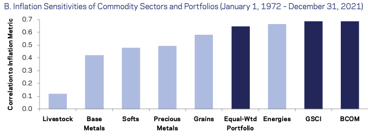
Chart B shows that over the past 50 years of price data, while inflation sensitivity varied across sectors, it was positive for all of them.
It was lowest for livestock and highest for energy (because of how much energy feeds into inflation).
And broad portfolios like the GSCI or BCOM index (whether equal- or production-weighted) had inflation sensitivities as high as energy (i.e., the highest individual sector).
Commodities have Delivered Higher Returns in Inflationary Environments
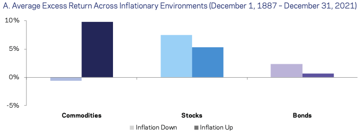
(Sources: Chicago Board of Trade, US Bureau of Labor Statistics, Commodity Systems Inc., S&P, Goldman Sachs, Bloomberg, and DataStream.)
(Chart A: Commodities is a hypothetical equal-weighted portfolio, which takes equal notional weights of all commodities in the basket at each point in time. The risk-free rate used to calculate the excess return is New York call money rates until 1889, the New York Times money rates until 1918, secondary market rates on the shortest term US bonds available until 1931, and T-bills thereafter. A rolling one-year average of the short-term rate is used. Aggregate global stocks returns are represented by GDP-weighted G6 (US, UK, Germany, Japan, Canada, and Australia) equities. Global bond returns are represented by GDP-weighted G6 government bonds. Inflation Up/Down refers to positive/negative 1-year inflation change (monthly with overlapping annual horizon).)
(Chart B: Inflation sensitivity is a contemporaneous partial correlation to a composite metric of inflation changes and surprises, controlling for growth exposure, based on quarterly data. Surprise is based on realization relative to forecasts of inflation from the Fed Survey of Professional Forecasters.)
Strategically Building a Better Commodities Portfolio
Most portfolios can see improved risk-adjusted returns from the addition of a commodities allocation, there are different ways for traders and investors to get access the asset class.
Passive commodity portfolios that track indices such as the GSCI and BCOM are likely to be the easiest and least expensive way.
Nonetheless, as we go into below, these indices are not well optimized because of their poor risk diversification and they lack risk management.
It would be up to the individual trader to risk manage any exposure to them.
This might include things like constraining the position size to reap the benefits without taking outsized risks, owning options (where available – the GSG ETF has option with the BCOM futures index (AIGCI*) does not).
Another approach to constructing a better strategic commodities portfolio differs from the passive indices in two main ways:
i) Better balancing of risks across sectors to improve diversification (e.g., less concentration in energy)
ii) Active management of exposures to target a more stable level of volatility in a portfolio
*AIGCI is constructed such that no single commodity can make up more than 15% of the index and its derived commodities (e.g., gasoline as it related to crude oil) cannot make up more than 25%.
Its targets can be found below.
Bloomberg Commodity Index Component Target Weights for 2026
| Group | Commodity | 2026 Target Weight (%) |
|---|---|---|
| Energy | Brent Crude Oil | 8.36 |
| Natural Gas | 7.20 | |
| WTI Crude Oil | 6.64 | |
| Low Sulphur Gas Oil | 2.89 | |
| ULS Diesel | 2.19 | |
| RBOB Gasoline | 2.15 | |
| Energy Total | 29.44 | |
| Grains | Corn | 5.53 |
| Soybeans | 5.36 | |
| Soybean Meal | 2.93 | |
| Soybean Oil | 2.82 | |
| Wheat | 2.72 | |
| HRW Wheat | 1.79 | |
| Grains Total | 21.15 | |
| Industrial Metals | COMEX Copper | 6.36 |
| LME Aluminum | 3.97 | |
| LME Zinc | 2.25 | |
| LME Nickel | 2.23 | |
| Lead | 0.95 | |
| Industrial Metals Total | 15.76 | |
| Precious Metals | Gold | 14.90 |
| Silver | 3.94 | |
| Precious Metals Total | 18.84 | |
| Softs | Sugar | 2.95 |
| Coffee | 2.91 | |
| Cocoa | 1.71 | |
| Cotton | 1.59 | |
| Softs Total | 9.17 | |
| Livestock | Live Cattle | 3.86 |
| Lean Hogs | 1.78 | |
| Livestock Total | 5.64 |
Better risk balance across commodity sectors
As seen below, the traditional commodity indices (i.e., GSCI and BCOM) have large risk allocations to energy commodities, coming in around 45 percent toward energy commodities (e.g., crude oil, gasoline, natural gas, heating oil).
This risk that has historically not been rewarded with a higher return in kind.
Traders can increase their risk-adjusted returns through improved diversification by better balancing their risks across commodity sectors.
Traditional Commodity Indices are Concentrated in Energies
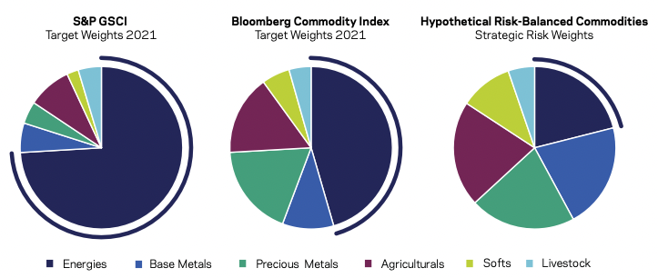
(Source: Bloomberg, AQR. Risk allocations based on 2021 target weights for the S&P GSCI and Bloomberg Commodity Indices, long-term strategic weights of a hypothetical risk-balanced commodities portfolio, and volatility and correlation estimates provided by AQR. There is no assurance that the target risk allocations will be achieved, and actual allocations may be significantly different than that shown here.)
In the hypothetical risk-balanced portfolio (shown on the right), every commodity sector contributes to risk and returns, but with no one sector dominating.
This is similar to the concepts we go over in our articles on balanced portfolios and how to better allocate among asset classes to achieve more return per each unit of risk taken on.
Higher-risk sectors, notably energy, are given smaller notional allocations while lower-risk sectors, such as precious metals, are given higher allocations relative to a traditional commodity index.
But even though it’s more diversified, this approach will have lower capacity (ability for institutional investors to deploy it in size) than allocating by liquidity or global production.
The potential benefits to this approach, however, are material.
Because each commodity has unique supply-and-demand characteristics, commodity sectors are less correlated than equity or fixed income sectors, which tend to be highly tied together.
For example, consumer staples stocks and technology stocks – even though their sources of cash flow are different – are 72 percent positively correlated, based on data from the XLY (Consumer Discret Sel Sect SPDR ETF) and XLK (Technology Select Sector SPDR ETF) ETFs that go back to December 1998.
So if diversifying across global equity markets is valuable, diversifying across commodity markets is even more valuable.
Targeting more stable risk through time
Concentrating risk in one or two sectors is best avoided, just as concentrating risk in one or two time periods can also cause problems for traders.
Spikes in risk historically exhibited by commodities can be managed by targeting a pre-specified level of volatility.
The chart below shows the realized volatility of a hypothetical risk-balanced commodity portfolio that is volatility-managed.
Instead of a fixed notional exposure to commodities, the notional exposure to commodities is adjusted daily using a short-term estimate of volatility.
The realized volatility of the risk-managed commodity portfolio will remain in a range much closer to its target.
On the other hand, the volatility of the Bloomberg Commodity Index (BCOM) will spike to much higher levels, especially during periods of higher market volatility (e.g., bear markets, geopolitical conflict).
At the same time, it will realize a low volatility during other times.
By keeping a steadier level of volatility, a portfolio with prudent risk management may experience less of the big ups and down that can cause portfolios problems and suffer less from negative tail events.
Volatility Targeting May Provide a Less Bumpier Ride
Annual Realized Volatility of Commodities Portfolios (January 1, 1991 – December 31, 2021)
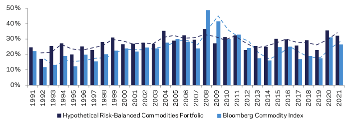
(Source: AQR, Bloomberg. Data using 3-day returns. Dotted lines are 2-period moving averages. Performance from January 1, 1991 through December 31, 2021 of a hypothetical risk-balanced commodities portfolio and the Bloomberg Commodity Index. Performance is in USD, gross of fees and transaction costs.)
These improvements, however, do not come without a cost.
A risk-targeted and risk-balanced portfolio requires the more frequent rebalancing of positions as risk levels change.
Moreover, it allocates larger portfolio weights to contracts that are less liquid relative to passive indices (e.g., energy tends to be more liquid than agriculture).
These features will lead to lower capacity (ability to do it in size) and higher turnover in addition to the tracking error to passive indices.
Performance using this approach will vary widely, with traditional approaches still outperforming significantly at times.
However, in the long term, for someone focused on risk-adjusted returns and getting returns in the most efficient way possible, the potential benefits to holding a risk-balanced and risk-targeted commodities portfolio outweigh these costs.
Commodity Fundamentals and Active Management
Beyond the above strategic commodities portfolio, there can be benefits to active commodity management.
This involves overweighting commodities with strong current fundamentals, rising trends, and positive carry.
Performance can be improved further through efficient trading and careful implementation, including the selection of futures contracts and roll management.
An overview of commodity fundamentals and active signals
Commodities can be thought of in a few different ways:
- alternative currencies (i.e., hard forms of currencies that have transactional value)
- stores of value
- a growth-sensitive asset class
- markets subject to their own supply and demand characteristics
Knowing the fundamental drivers within each commodity market provides investors the opportunity to actively tilt a portfolio toward commodities that have a greater likelihood of outperforming in the short term.
For example, low or falling inventories may indicate that supply is too low, and lead to rising prices. On the other hand, rising inventories may indicate falling demand.
Seasonal patterns also matter in commodity markets.
Natural gas is well-known for this. Demand in the colder winter months often leads to predictably higher seasonable prices in November, December, January, and February.
Agricultural commodities also tend to see a large supply come forward during certain months and enter the market during harvest seasons in the northern hemisphere (where about 90 percent of the world’s population lives).
This tends to lower their prices because of the abundance during these months and increase hedging demands on lower prices.
To the extent these seasonal effects lead to changes in the risk premia of commodities, traders may want to incorporate them into their allocation process.
Macroeconomic data can provide insight into the demand for commodities, since global economic growth, inflation (which may be caused by commodities), and exchange rates are important feed-ins into commodity prices.
By looking at each commodity’s global consumption profile, traders may be able to understand which commodities will benefit or suffer most from changes in the economic health of the major commodity-consuming countries.
For example, Asia accounts for nearly 60 percent of global copper consumption because it’s a common building material and Asia is building a lot more than North America and Europe.
But their incomes aren’t as high so they only consume 32 percent of global crude oil consumption.
Accordingly, copper is likely to benefit more than oil from strong Asian growth.
Certain commodities are linked economically and this gives rise to relative value bets.
For instance, the fundamental relationship between the prices of crude oil, heating oil, and gasoline is known as the “crack spread”.
This references the process of refining crude oil into other products, which is often called “cracking”.
If the crack spread narrows too much, then refineries will slow their production of gasoline and schedule maintenance to protect profit margins.
This, in turn, will reduce the demand for crude oil and supply of products, which effectively forms a type of self-correcting feedback loop that should eventually push things back into equilibrium.
On the other hand, if the crack spread gets too wide, then refineries will be incentivized to increase production to capitalize on the larger refining margins, which will push crude oil up and again push prices back toward equilibrium.
A trader who analyzes the crack spread can potentially profit from this relationship by trading on the prices of crude relative to its products.
Carry in commodities
The concept of carry also applies to commodity futures.
Though carry is most common in currency markets, the analogous concept in commodity markets is roll yield.
This refers to a commodity futures contract having a positive carry if the futures price is below the current spot price (i.e., the current price) of the commodity.
The shape of the yield curve will be downward sloping, which is called backwardation.
It is common in markets where there’s a shortfall of supply relative to demand and prices are expected to keep increasing as a result, sometimes called a supercycle if it goes on for years.
In this case, the owner of that contract will earn carry as the futures price approaches the spot price over time.
But naturally, there is no guarantee that the expected carry will be earned. The spot price can change.
Just as someone having carry on a currency can see the exchange rate move in an unfavorable way or someone who owns a dividend stock may see the price fall by more than the yield they’re receiving.
But commodities with higher carry have historically earned higher returns.
Trend and momentum
Trend or momentum signals are another predictor of commodity returns.
Commodities tend to move in trends. When commodities have been increasing (or declining) in price over the past year, they have historically tended to continue in line with the trend.
Price momentum tends to work in commodity futures for the same reason it works in other asset classes: Investors and traders tend to anchor their views on prior prices in the near term and do not fully adjust prices to reflect new fundamentals, leading to a reaction that is not commensurate.
For example, if traders have been used to seeing oil being under $100 over the course of their lives or careers, then $100+ oil may seem very high or even impossible.
But supply and demand may change that make the price very realistic in some circumstances.
And in some cases, traders and investors tend to overreact to price moves due to herding tendencies, which can also lead to price trends.
Market participants can benefit from these trends by tactically overweighting commodities with positive price trends, and underweighting commodities with negative price trends.
The chart below summarizes active investment themes in commodity markets. These can be applied in absolute return strategies, long-biased, and long-only portfolios.
Active Investment Themes in Commodity Markets
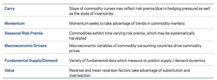
(Source: AQR)
A passive equity index is close to a so-called “buy and hold” portfolio.
By contrast, a “passive” commodity futures investment must trade regularly (or buy an ETF, where the “roll” is done for you).
The trader must exit each futures contract before expiry or accept physical delivery of the commodity.
In order to maintain exposure without taking delivery, the manager must “roll” the position.
In other words, they need to exit the contract that is about to expire and enter a contract of a later maturity in its place.
Standard commodity indices will roll on a fixed schedule.
Accordingly, they are vulnerable to traders who position themselves ahead of this predictable flow. By buying the longer contracts ahead of time and selling them to passive index holders at a higher price.
A number of other passive commodity portfolios have attempted to create value to the space by avoiding this by holding contracts with later expiry dates, which are called “deferred roll”.
But the advantages of this simple approach have diminished.
A different and more sophisticated approach that involves using return and cost forecasts to dynamically manage the process has provided a more sustainable advantage, as shown below.
Contract Selection Matters
Hypothetical Dynamic Roll May Offset Declining Premium to Deferred Roll over GSCI Roll (January 1, 2007 – December 31, 2021)
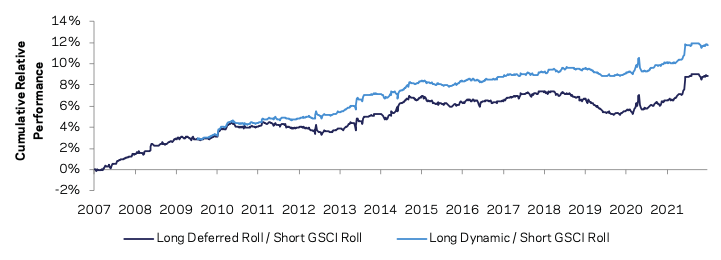
(Source: AQR, Bloomberg. Multiplies commodity weights used in a hypothetical risk-balanced commodities portfolio (described in the Appendix) by dynamically rolled commodity returns, deferred GSCI rolls, and standard GSCI rolls. Assumes 18% risk-targeted exposure to commodities.)
Conclusion
A long-biased passive investment in commodity futures may improve a traditional stocks and bonds asset portfolio by adding diversification and helping to preserve real value in periods of rising inflation or higher inflation volatility.
This article shows how traders can build a better strategic commodities portfolio by risk-balancing across commodity sectors and targeting steady volatility over time.
Performance may also be improved further through active signals based on commodity fundamentals, macroeconomic data such as growth and inflation, price trends, and roll management.
The chart below shows that this performance improvement has also been available for a hypothetical risk-balanced commodities portfolio over a 30-year history.
The last two columns show that strategic design choices and active tilts both contributed to this outperformance.
Putting It All Together
Hypothetical Risk-Balanced Commodities vs. Passive Index (January 1, 1991 – December 31, 2021)
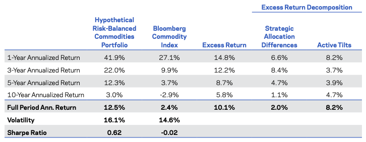
(Source: AQR. Performance from January 1, 1991 through December 31, 2021 of a hypothetical risk-balanced commodities portfolio (described in the Appendix) and the Bloomberg Commodity Index. Performance is in USD, gross of fees and transaction costs. Past performance is not a reliable indicator of future performance. Please read important disclosures in the Appendix. The risk free rate used to calculate the Sharpe ratios is the ICE BofAML 3-month U.S. Treasury Bill.)
Appendix: Data and Methodology
Data
Commodity contract prices are from Chicago Board of Trade for the period before 1951, Commodity Systems Inc. for 1951-2012, and Bloomberg for 2012-2021.
Rolled return series for platinum, aluminum, copper, lead, nickel, tin, and zinc are from S&P, Goldman Sachs, Bloomberg, and DataStream.
Results are for equal dollar-weighted portfolio, which takes equal notional weights of all commodities in the commodity basket at each point in time.
The risk free rate used to calculate the Sharpe ratios is New York call money rates until 1889, the New York Times money rates until 1918, secondary market rates on the shortest term U.S.bonds available until 1931 and T-bills thereafter.
A rolling one-year average of the short-term rate is used. Aggregate global stocks returns are represented by GDP-weighted G6 (US, UK, Germany, Japan, Canada, and Australia) equities. Global bond returns are represented by GDP-weighted G6 government bonds. Global 60/40 is based on a 60% Global Stocks and 40% Global Bonds.
Inflation data are from George F. Warren and Frank A. Pearson, Gold and Prices (New York: John Wiley and Sons, 1935) for the period before 1913 and the U.S. Bureau of Labor Statistics for 1913-2021.
Hypothetical Risk-Balanced Commodities Portfolio
The risk-balanced commodities portfolio studied herein rebalances monthly and is risk- balanced across the following 26 commodities in 6 sectors:
- Agriculture (Corn, Soybeans, Wheat, Soybean Meal, Soybean Oil)
- Softs (Coffee, Cocoa, Cotton, Sugar)
- Energies (WTI Crude, Brent Crude, Gas Oil, Gasoline, Heating Oil, Natural Gas)
- Livestock (Live Cattle, Feeder Cattle, Lean Hogs)
- Precious Metals (Gold, Silver)
- Base Metals (Aluminum, Platinum, Copper, Nickel, Zinc, Lead)
- (It gives equal notional weight to commodities within each sector.)
The portfolio targets a constant volatility of 18 percent at each monthly rebalance, subject to a risk reduction process.
The portfolio volatility is estimated using a combination of individual volatilities and pair-wise correlations.
The individual volatilities are calculated using historical daily returns, weighted exponentially with a 60-day center of mass.
Correlation estimates are calculated using 5-day overlapping returns (to account for different market close times), exponentially weighted with a 150-day center of mass.
Inflation Sensitivity Methodology
The metric combines two measures of changing expectations for US inflation:
1. year-on-year CPI inflation minus CPI for the previous 1-year period (“change”)
2. year-on-year CPI inflation minus 1-year forecast at the start of the period (“surprise”)
We combine the two measures (standardized so they have equal influence) to reduce noise in either one.
We construct a corresponding metric for US GDP growth, as a control variable.
Sensitivity is a contemporaneous partial correlation to inflation metric, based on quarterly overlapping year-on-year periods, to avoid seasonal effects and mitigate the role of publication lags.
Other Portfolios
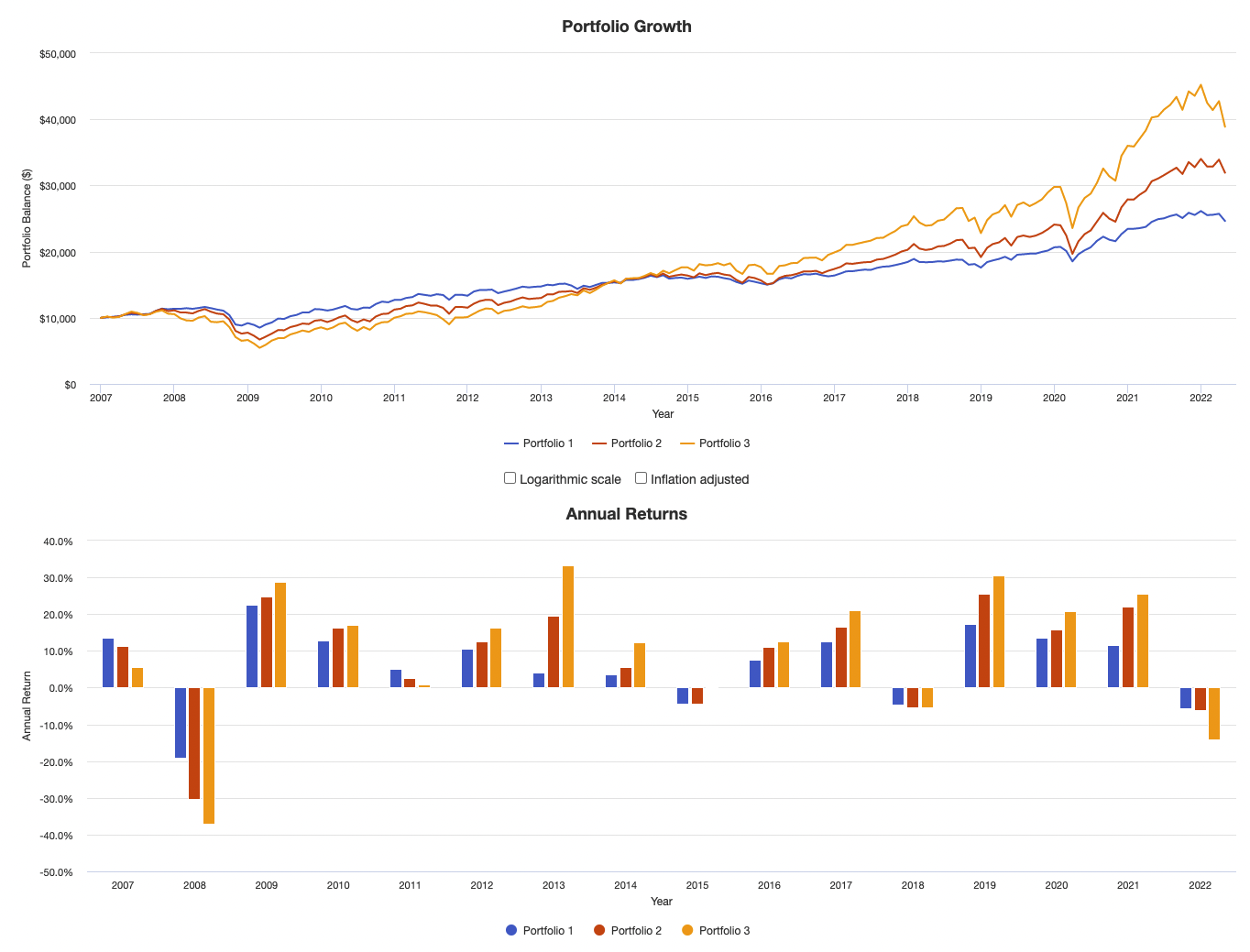
We can also check other allocations to see how well commodities have helped them historically.
Let’s take a look at the following:
Portfolio 1: Most diversified
Portfolio 2: Mostly in stocks, but with 10 percent allocations to TIPS (US inflation-indexed government bonds), gold, and commodities.
Portfolio 3: Stocks only
Portfolio Allocations
| Asset Class | Allocation |
|---|---|
| US Stock Market | 30.00% |
| TIPS | 35.00% |
| Gold | 10.00% |
| Commodities | 5.00% |
| Global ex-US Stock Market | 5.00% |
| Global Bonds (Unhedged) | 5.00% |
| Emerging Markets | 5.00% |
| Long-Term Tax-Exempt | 5.00% |
| Asset Class | Allocation |
|---|---|
| US Stock Market | 70.00% |
| TIPS | 10.00% |
| Gold | 10.00% |
| Commodities | 10.00% |
| Asset Class | Allocation |
|---|---|
| US Stock Market | 100.00% |
Portfolio Returns
| Portfolio | Initial Balance | Final Balance | CAGR | Stdev | Best Year | Worst Year | Max. Drawdown | Sharpe Ratio | Sortino Ratio | Market Correlation |
|---|---|---|---|---|---|---|---|---|---|---|
| Portfolio 1 | $10,000 | $24,633 | 6.06% | 8.68% | 22.55% | -19.13% | -26.90% | 0.63 | 0.92 | 0.87 |
| Portfolio 2 | $10,000 | $31,932 | 7.87% | 12.93% | 25.61% | -30.29% | -40.85% | 0.59 | 0.85 | 0.97 |
| Portfolio 3 | $10,000 | $38,878 | 9.26% | 16.01% | 33.35% | -37.04% | -50.89% | 0.58 | 0.85 | 1.00 |
Performance
Drawdowns
Expectedly, the most diversified portfolio does best in terms of drawdowns while the least diversified does worst.
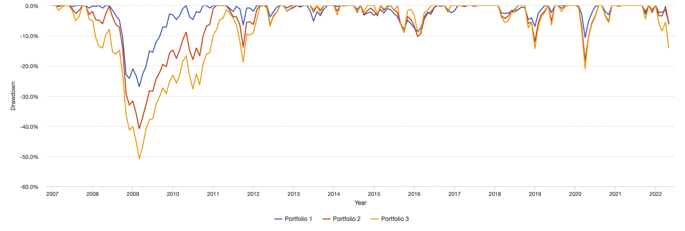
Drawdowns for Portfolio 1
| 1 | Jun 2008 | Feb 2009 | 9 months | Apr 2010 | 1 year 2 months | 1 year 11 months | -26.90% |
| 2 | Feb 2020 | Mar 2020 | 2 months | Jul 2020 | 4 months | 6 months | -10.60% |
| 3 | Sep 2014 | Jan 2016 | 1 year 5 months | Jul 2016 | 6 months | 1 year 11 months | -8.68% |
| 4 | Feb 2018 | Dec 2018 | 11 months | Apr 2019 | 4 months | 1 year 3 months | -6.93% |
| 5 | May 2011 | Sep 2011 | 5 months | Jan 2012 | 4 months | 9 months | -6.42% |
| 6 | Jan 2022 | Apr 2022 | 4 months | -5.74% | |||
| 7 | May 2013 | Jun 2013 | 2 months | Oct 2013 | 4 months | 6 months | -5.20% |
| 8 | May 2010 | Jun 2010 | 2 months | Sep 2010 | 3 months | 5 months | -4.65% |
| 9 | May 2012 | May 2012 | 1 month | Aug 2012 | 3 months | 4 months | -3.78% |
| 10 | Sep 2020 | Oct 2020 | 2 months | Nov 2020 | 1 month | 3 months | -3.08% |
| Worst 10 drawdowns included above | |||||||
Drawdowns for Portfolio 2
| 1 | Nov 2007 | Feb 2009 | 1 year 4 months | Jan 2011 | 1 year 11 months | 3 years 3 months | -40.85% |
| 2 | Jan 2020 | Mar 2020 | 3 months | Jul 2020 | 4 months | 7 months | -18.35% |
| 3 | May 2011 | Sep 2011 | 5 months | Feb 2012 | 5 months | 10 months | -13.84% |
| 4 | Oct 2018 | Dec 2018 | 3 months | Apr 2019 | 4 months | 7 months | -12.02% |
| 5 | Jun 2015 | Jan 2016 | 8 months | Jul 2016 | 6 months | 1 year 2 months | -10.30% |
| 6 | Apr 2012 | May 2012 | 2 months | Aug 2012 | 3 months | 5 months | -6.43% |
| 7 | Jan 2022 | Apr 2022 | 4 months | -6.11% | |||
| 8 | May 2019 | May 2019 | 1 month | Jun 2019 | 1 month | 2 months | -5.20% |
| 9 | Sep 2020 | Oct 2020 | 2 months | Nov 2020 | 1 month | 3 months | -5.20% |
| 10 | Feb 2018 | Mar 2018 | 2 months | Jul 2018 | 4 months | 6 months | -4.27% |
| Worst 10 drawdowns included above | |||||||
Drawdowns for Portfolio 3
| 1 | Nov 2007 | Feb 2009 | 1 year 4 months | Mar 2012 | 3 years 1 month | 4 years 5 months | -50.89% |
| 2 | Jan 2020 | Mar 2020 | 3 months | Jul 2020 | 4 months | 7 months | -20.89% |
| 3 | Oct 2018 | Dec 2018 | 3 months | Apr 2019 | 4 months | 7 months | -14.28% |
| 4 | Jan 2022 | Apr 2022 | 4 months | -14.01% | |||
| 5 | Jun 2015 | Sep 2015 | 4 months | May 2016 | 8 months | 1 year | -8.88% |
| 6 | Apr 2012 | May 2012 | 2 months | Aug 2012 | 3 months | 5 months | -6.85% |
| 7 | May 2019 | May 2019 | 1 month | Jun 2019 | 1 month | 2 months | -6.45% |
| 8 | Sep 2020 | Oct 2020 | 2 months | Nov 2020 | 1 month | 3 months | -5.65% |
| 9 | Feb 2018 | Mar 2018 | 2 months | Jul 2018 | 4 months | 6 months | -5.64% |
| 10 | Jun 2007 | Jul 2007 | 2 months | Oct 2007 | 3 months | 5 months | -5.02% |
| Worst 10 drawdowns included above | |||||||
Annual Returns
| 2007 | 4.08% | 13.64% | $11,364 | 11.21% | $11,121 | 5.49% | $10,549 | 5.49% | 11.59% | 30.45% | 31.62% | 15.52% | 9.26% | 38.90% | 2.54% |
| 2008 | 0.09% | -19.13% | $9,191 | -30.29% | $7,752 | -37.04% | $6,642 | -37.04% | -2.85% | 4.92% | -45.75% | -44.10% | -2.68% | -52.81% | -4.87% |
| 2009 | 2.72% | 22.55% | $11,263 | 24.69% | $9,666 | 28.70% | $8,548 | 28.70% | 10.80% | 24.03% | 11.22% | 36.73% | 17.17% | 75.98% | 14.08% |
| 2010 | 1.50% | 12.71% | $12,695 | 16.23% | $11,235 | 17.09% | $10,009 | 17.09% | 6.17% | 29.27% | 7.17% | 11.12% | 11.24% | 18.86% | 1.50% |
| 2011 | 2.96% | 5.04% | $13,334 | 2.63% | $11,530 | 0.96% | $10,105 | 0.96% | 13.23% | 9.57% | -3.28% | -14.56% | 9.20% | -18.78% | 10.69% |
| 2012 | 1.74% | 10.49% | $14,733 | 12.66% | $12,989 | 16.25% | $11,748 | 16.25% | 6.77% | 6.60% | -0.58% | 18.14% | 7.42% | 18.64% | 8.08% |
| 2013 | 1.50% | 4.05% | $15,331 | 19.44% | $15,513 | 33.35% | $15,666 | 33.35% | -8.92% | -28.33% | -1.83% | 15.04% | -5.04% | -5.19% | -2.95% |
| 2014 | 0.76% | 3.68% | $15,895 | 5.57% | $16,377 | 12.43% | $17,613 | 12.43% | 3.83% | -2.19% | -32.96% | -4.24% | 2.37% | 0.42% | 11.07% |
| 2015 | 0.73% | -4.29% | $15,213 | -4.45% | $15,648 | 0.29% | $17,664 | 0.29% | -1.83% | -10.67% | -34.06% | -4.38% | -3.57% | -15.47% | 3.97% |
| 2016 | 2.07% | 7.70% | $16,384 | 11.04% | $17,376 | 12.53% | $19,878 | 12.53% | 4.52% | 8.03% | 10.12% | 4.65% | 4.25% | 11.50% | 0.62% |
| 2017 | 2.11% | 12.49% | $18,430 | 16.69% | $20,276 | 21.05% | $24,063 | 21.05% | 2.81% | 12.81% | 3.89% | 27.40% | 9.21% | 31.15% | 6.43% |
| 2018 | 1.91% | -4.59% | $17,584 | -5.41% | $19,179 | -5.26% | $22,798 | -5.26% | -1.49% | -1.94% | -13.88% | -14.44% | -3.82% | -14.71% | 0.90% |
| 2019 | 2.29% | 17.42% | $20,647 | 25.61% | $24,090 | 30.65% | $29,785 | 30.65% | 8.06% | 17.86% | 15.62% | 21.43% | 6.67% | 20.13% | 8.49% |
| 2020 | 1.36% | 13.47% | $23,428 | 15.79% | $27,893 | 20.87% | $36,001 | 20.87% | 10.90% | 24.81% | -23.94% | 11.16% | 9.77% | 15.05% | 6.21% |
| 2021 | 7.04% | 11.55% | $26,134 | 21.93% | $34,010 | 25.59% | $45,214 | 25.59% | 5.56% | -4.15% | 38.77% | 8.61% | -3.55% | 0.73% | 2.26% |
| 2022 | 3.12% | -5.74% | $24,633 | -6.11% | $31,932 | -14.01% | $38,878 | -14.01% | -4.89% | 3.48% | 38.40% | -12.00% | -8.54% | -11.45% | -9.93% |
Portfolio return and risk metrics
| Arithmetic Mean (monthly) | 0.52% | 0.70% | 0.85% |
|---|---|---|---|
| Arithmetic Mean (annualized) | 6.46% | 8.78% | 10.67% |
| Geometric Mean (monthly) | 0.49% | 0.63% | 0.74% |
| Geometric Mean (annualized) | 6.06% | 7.87% | 9.26% |
| Standard Deviation (monthly) | 2.51% | 3.73% | 4.62% |
| Standard Deviation (annualized) | 8.68% | 12.93% | 16.01% |
| Downside Deviation (monthly) | 1.70% | 2.56% | 3.15% |
| Maximum Drawdown | -26.90% | -40.85% | -50.89% |
| Stock Market Correlation | 0.87 | 0.97 | 1.00 |
| Beta(*) | 0.47 | 0.78 | 1.00 |
| Alpha (annualized) | 1.48% | 0.48% | 0.00% |
| R2 | 75.31% | 93.75% | 100.00% |
| Sharpe Ratio | 0.63 | 0.59 | 0.58 |
| Sortino Ratio | 0.92 | 0.85 | 0.85 |
| Treynor Ratio (%) | 11.62 | 9.77 | 9.38 |
| Calmar Ratio | 0.81 | 0.72 | 0.62 |
| Active Return | -3.20% | -1.39% | 0.00% |
| Tracking Error | 9.51% | 4.76% | 0.00% |
| Information Ratio | -0.34 | -0.29 | N/A |
| Skewness | -1.16 | -0.95 | -0.65 |
| Excess Kurtosis | 5.65 | 3.37 | 1.56 |
| Historical Value-at-Risk (5%) | -3.36% | -6.09% | -7.99% |
| Analytical Value-at-Risk (5%) | -3.60% | -5.44% | -6.75% |
| Conditional Value-at-Risk (5%) | -5.67% | -8.54% | -10.21% |
| Upside Capture Ratio (%) | 45.77 | 76.40 | 100.00 |
| Downside Capture Ratio (%) | 42.19 | 76.71 | 100.00 |
| Safe Withdrawal Rate | 8.68% | 8.52% | 8.49% |
| Perpetual Withdrawal Rate | 3.59% | 5.24% | 6.47% |
| Positive Periods | 119 out of 184 (64.67%) | 117 out of 184 (63.59%) | 123 out of 184 (66.85%) |
| Gain/Loss Ratio | 0.97 | 0.95 | 0.80 |
| * US stock market is used as the benchmark for calculations. Value-at-risk metrics are based on monthly values. | |||
Monthly Correlations
Correlations for the portfolio assets:
| US Stock Market | 1.00 | 0.21 | 0.06 | 0.51 | 0.89 | 0.40 | 0.78 | 0.15 | 0.87 | 0.97 | 1.00 |
| TIPS | 0.21 | 1.00 | 0.51 | 0.17 | 0.30 | 0.69 | 0.34 | 0.46 | 0.57 | 0.33 | 0.21 |
| Gold | 0.06 | 0.51 | 1.00 | 0.22 | 0.19 | 0.49 | 0.27 | 0.17 | 0.46 | 0.26 | 0.06 |
| Commodities | 0.51 | 0.17 | 0.22 | 1.00 | 0.60 | 0.34 | 0.57 | -0.04 | 0.63 | 0.65 | 0.51 |
| Global ex-US Stock Market | 0.89 | 0.30 | 0.19 | 0.60 | 1.00 | 0.58 | 0.93 | 0.19 | 0.90 | 0.91 | 0.89 |
| Global Bonds (Unhedged) | 0.40 | 0.69 | 0.49 | 0.34 | 0.58 | 1.00 | 0.56 | 0.46 | 0.69 | 0.50 | 0.40 |
| Emerging Markets | 0.78 | 0.34 | 0.27 | 0.57 | 0.93 | 0.56 | 1.00 | 0.20 | 0.86 | 0.82 | 0.78 |
| Long-Term Tax-Exempt | 0.15 | 0.46 | 0.17 | -0.04 | 0.19 | 0.46 | 0.20 | 1.00 | 0.29 | 0.15 | 0.15 |