What Determines Bond Yields?

We look into the determinants behind “risk-free” government bond yields.

At its core, bond yields are shaped by a trio of elements:

1. The prevailing short-term interest rate
2. Anticipated future interest rates
3. A term premium

While sovereign credit risk plays a role in many nations, for the scope of this discussion, we’ll set it aside, focusing instead on countries that are reliably expected to honor their nominal debts (i.e., reserve currency countries).

Central banks predominantly dictate the short-term interest rate and its foreseeable trajectory.

Yet, when we look at long-term interest rates and term premia, external factors, beyond policy decisions, come into play.

Monetary policy, with its basic triad of tools – traditional interest rate tweaks, quantitative easing (QE), and forward guidance – responds to economic indicators and molds conditions from short-term maturities to longer-duration yields.

However, both theory and empirical evidence suggest that external factors, detached from monetary policy, have a profound impact on yields, particularly for bonds with extended maturities.

For instance, 10-year Treasuries consistently align with shifts in growth and inflation projections over that period.

A decline in nominal growth expectations typically heralds a dip in bond yields.

While the actions of central banks sway bond yields, it’s the economic fundamentals that steer the bond markets.

Key Takeaways – What Determines Bond Yields?

• Central banks heavily influence bond yields through monetary tools.
• Non-policy factors, like growth expectations, impact long-term yields.
• Term premia reflect risks and demand for long-duration bonds.

Intro to Bond Yields

Let’s look at an overview.

What Determines Bond Yields?

Bond yields, especially those of long-duration government bonds, are influenced by a myriad of factors.

For traders and investors in bond markets, understanding these determinants is critical for trading well, be it in bond futures, ETFs, or the actual bonds.

Key Determinants of Bond Yields

The key determinants of bond yields include:

Short-term Interest Rates

The current short-term interest rate, predominantly controlled by the central bank, is a significant factor.

This rate is largely influenced by nominal growth rates, which include real growth and inflation.

The “Taylor Rule” describes how central banks set this rate, primarily based on unemployment and inflation rates.

Expected Future Interest Rates

These are shaped by monetary policy.

Central banks use forward guidance to signal the anticipated path of monetary policy, which in turn affects long-term bond yields.

Term Premia

This is the extra compensation investors expect for holding a long-term bond over a short-term one.

It’s influenced by:

• Risk aversion levels
• Inflation certainty fluctuations
• Supply and demand dynamics of government debt, driven by entities like central banks, pension funds, corporations, and more

Monetary Policy’s Role

Central banks’ actions, such as purchasing longer-duration assets (e.g., bonds, corporate credit), can decrease term premia, leading to reduced bond yields.

This strategy, known as quantitative easing (QE), began as a response to the 2008 financial crisis.

Other tools like average inflation targeting, operation twist, and yield curve control also influence bond yields.

Macroeconomic Forces

Long-term inflation expectations play a pivotal role. Domestic investors gauge inflation to determine the desired bond yield.

For instance, if inflation is at 3%, they’d expect a bond yield of at least 3% to maintain their real wealth (i.e., buying power).

However, foreign investors prioritize currency effects over local inflation rates.

Other Influential Factors

• Trend growth.
• Long-term inflation expectations.
• Inflation uncertainty.
• External demand.
• Regulatory considerations.
• Risk aversion levels.

Despite central bank interventions, fundamental forces remain influential.

Even without central bank actions, low economic growth would likely result in low yields.

Both monetary and non-monetary factors can sway long-term interest rates and term premia.

Risks and Considerations

Bond risks are multifaceted. While they were reliable hedges from 1981-2020, their efficacy has diminished due to low yields.

If inflation expectations rise, it could impact both stocks and bonds. Declining long-term growth expectations could benefit bonds but adversely affect stocks.

Although bonds offer diversification, their low yields limit their income generation potential.

Breaking down bond yields

A bond yield is the average expected interest rate over its life plus a term premium. 

This isn’t just a simple interest rate, though. Added to this expected rate is what’s known as a “term premium.”

The term premium compensates traders/investors for the potential risks associated with holding a bond over a longer period, such as inflation or interest rate changes.

In essence, the bond yield carries both the predictable returns from the bond and the additional compensation for the uncertainties of the future.

The Expectations Hypothesis

Theory is used to help understand the policy and non-policy drivers of bond yields in more depth. 

The expectations hypothesis (EH) is a basic theory of the yield curve. The EH asserts that term premia hold constant over time, but may vary based on maturity. 

At its core, the EH posits that term premia, while remaining constant over time, can exhibit variations depending on the bond’s maturity.

In simpler terms, while the compensation for potential risks might stay steady over a period, it could differ based on the bond’s duration or time to maturity.

By understanding the EH, we gain a clearer perspective on the underlying factors that shape and influence bond yields across different maturities.

Understanding Interest Rates and Bond Yields

To understand bond yields, it’s essential to understand the driving forces behind interest rate changes.

Central Banks and Interest Rates

• Central banks in developed markets predominantly control the short-term interest rate, typically an “overnight” rate or a three-month rate.
• This rate adjustment is the primary method for managing monetary policy.
• Central banks operate with mandates, which often include:
  • Maintaining low and stable inflation. Some, like the ECB, focus solely on inflation.
  • Ensuring low unemployment. For instance, the Fed targets both inflation and unemployment and has an unofficial mandate for financial stability.

Economic Frameworks and Models

Central banks utilize various models to understand economic events and their impact:

• Aggregate Demand (AD) and Aggregate Supply (AS): These represent the real economy (goods and services) and the financial economy (money and credit), respectively.
• Taylor Rule (TR): A model showcasing how central banks determine interest rates.
• Expectations Hypothesis (EH): This links bond yield to current and expected interest rates.

Aggregate Demand and the Output Gap

• The output gap is a critical concept, representing the difference between:
  • The economy’s potential output at “full employment.”
  • The current output level.
• Policymakers and traders monitor the unemployment rate and job reports, comparing the current rate to the “natural rate of unemployment” or “NAIRU.”
• The real yield (nominal yield minus inflation expectations) plays a significant role in the aggregate demand relationship.
• The output gap influences central bank policies. A high gap might lead to more lenient monetary policies, while a low gap with rising inflation might result in tighter policies.
• The real yield affects various borrowing and savings rates, impacting asset values, termed the “wealth effect.”

Aggregate Supply and Inflation

• Aggregate supply connects inflation levels with expected inflation and the output gap.
• Expected inflation plays a role in actual inflation due to “inflation psychology.” If consumers expect prices to rise, they’re more likely to spend, leading to actual price increases.
• Companies often adjust wages based on inflation expectations. Higher expected inflation can lead to workers negotiating for increased wages.
• Inflation correlates with the output gap. A positive output gap can lead to price increases, while a negative one might result in price reductions.

Monetary Policy and Its Influence on Bond Yields

The AD-AS-TR-EH framework covered above integrates both conventional and unconventional monetary policies.

Among these, the adjustment of short-term interest rates stands out as the most traditional method, and it’s this aspect we’ll look into.

Central Bank’s Influence on Macroeconomic Variables

Central banks wield a degree of influence over short-term inflation and the output gap.

But how exactly do they exert this influence by tweaking the short-term interest rate?

This process is encapsulated in what’s termed the “monetary transmission mechanism.”

Monetary Transmission Mechanism Explained

1. Setting the Short-Term Interest Rate: Within the AD-AS-TR-EH model, the short-term interest rate doesn’t directly affect macroeconomic variables. Its primary influence is on the nominal yield of long-term bonds.
2. Influence on Real Yields: Given that long-term inflation expectations are generally stable, alterations in long-term bonds effectively translate to changes in real yields.
3. Impact on Output Gap and Inflation: Through the aggregate demand (AD) component, shifts in real yields influence the output gap. Concurrently, via the aggregate supply (AS) component, variations in the output gap affect inflation levels.
4. Achieving Mandated Objectives: By modulating the nominal interest rate, central banks can steer the macroeconomic variables they are tasked with overseeing, namely inflation and output (represented by the output gap).

Determining the Interest Rate

• Data-Driven Decisions: Central banks continually monitor data on inflation and output to make informed decisions.
• Inflation Targeting: Every central bank has an inflation benchmark. If actual inflation falls below this target, the typical response is to reduce the interest rate or maintain a low rate over an extended duration. Conversely, when inflation surpasses the target, the interest rate is increased to temper both output and inflation.
• Output Monitoring: Some central banks also have the responsibility of monitoring output. If the output gap is negative (indicating that the current output is lagging behind its potential), the central bank is inclined to decrease the interest rate or sustain it at a low level to stimulate output. However, if the output gap is positive (signifying that the current output exceeds its potential), the central bank might opt to increase the interest rate to prevent potential inflationary pressures.

The Taylor Rule

In 1993, economist John Taylor introduced a foundational framework for determining an economy’s optimal interest rate.

This framework, known as the Taylor Rule, is widely utilized by economists, policymakers, and traders to gauge the ideal interest rate, given its alignment with economic data.

The Taylor Rule is constructed as follows:

i = r* + π + bπ (π – π*) + bY (Y – Y*)

• π – π* is called the “inflation gap”. This is the difference between the current inflation rate, π, and the central bank’s inflation target, π*. 
• Y – Y* is the output gap. This is the difference between output Y, and the full employment level of output Y*. 
• bπ is a positive number, so the Taylor Rule does a good job of showing that the central bank should set a higher interest rate when inflation exceeds its target and a lower interest rate when inflation is below its target. 
• bY is also greater than zero, so the Taylor Rule asserts that the interest rate should be higher when the output gap is positive (an expansion) and lower when the output gap is negative (a contraction).

Implications of the Taylor Rule

The formula suggests:

• When inflation surpasses its target, the central bank should raise the interest rate.
• When the output gap is positive (indicating economic expansion), the interest rate should be higher, and vice versa for a negative output gap (indicating economic contraction).

What about r*+π, the first two terms in the Taylor Rule formula?

r* (pronounced “r star”) is the equilibrium real interest rate and π is standard economics notation for inflation. In other words, r-star plus inflation is the nominal interest rate.

To understand the Taylor Rule as a real interest rate you can subtract inflation from both sides of the equation:

Real Interest Rate = i – π = r* + bπ (π – π*) + bY(Y – Y*)

(To be more technically accurate, inflation expectations over X years matched to the maturity of the interest rate should be subtracted – e.g., 10-year inflation expectations subtracted from the 10-year bond yield – but realized inflation is a quality stand-in measure.)

The Taylor Rule would prescribe a real interest rate above r* when the inflation gap or output gap is positive (i.e., overheating economy), and a real interest rate below r* when the inflation gap or output gap is negative (i.e., sluggish economy). 

When both are zero the Taylor Rule would prescribe a real interest rate equal to r*. 

Accordingly, r* describes the “natural rate of interest” or the rate at which an economy would have neutral monetary policy when there’s no inflation or output gap. 

In other words, the real interest rate is consistent with output equal to potential output (i.e., full employment) and stable inflation.

The real interest rate, in practice, depends on the output gap and inflation gap via the Taylor Rule. 

Similarly, short-run expected future real interest rates depend on forecasts of the output gap and inflation gap. 

What about long-run expectations of the real interest rate?

As time horizons lengthen, cyclical forces become less important. 

As we’ve explained in other articles, productivity trends are the biggest determinant of economic growth and performance over the long-term.

In the short-run, the credit cycles that monetary policy helps control matter more. 

Cyclical forces matter less as time goes on and monetary policy is neutral on net. 

Accordingly, the expected future real interest rate, eventually comes to r*. 

So, long-term expectations of the real interest rate are anchored by r*. Likewise, long-term expectations of the nominal interest rate are anchored by r* + πLT, where πLT denotes long-term inflation expectations. 

Because long-duration bond yields are heavily determined by expected future interest rates, their yields and valuations should be more sensitive to changes r* + πLT relative to shorter-term bonds.

In general, all long-duration assets (including long-duration bonds and stocks) and more sensitive to fluctuations in r* + πLT.

In a later section of this article, we show that long-maturity yields tend to move in lockstep with changes in the natural rate of interest and long-term inflation expectations.

Term premia

The term premium is the additional compensation that traders and bond investors require to hold to maturity a long-maturity bond versus rolling over short-maturity debt (e.g., three-month Treasury bills). 

Term premia are positive over time and rise with maturity. Namely, investors will typically require extra yield to hold long-duration bonds over short-duration bonds. 

Term premia at any given point cannot be found exactly. The yield curve finds average term premia at a point in time. Estimating exact term premia is done by some economists (e.g., Kim and Wright (2005), the ACM model kept by the New York Fed). But they have large standard errors.

The general idea here is to understand the drivers of term premia.

Term premia encompass all factors that influence a bond’s yield outside the currency interest rate and expectations of future interest rate. 

The biggest drivers are:

• Changes in perceived risk
• Changes in supply and demand

Risk

Risk plays a big role in determining bond yields.

When traders/investors perceive higher risks associated with a particular bond or the broader economic environment, they demand a higher yield as compensation.

This risk can arise from various factors:

• Credit Risk: The possibility that the bond issuer might default on their obligations.
• Interest Rate Risk: The potential for bond prices to fall due to rising interest rates.
• Reinvestment Risk: The risk that bondholders might have to reinvest their funds at lower rates if their bonds mature during a period of declining interest rates.
• Liquidity Risk: The risk that an investor might not be able to sell a bond at a fair price quickly.

In essence, the greater the perceived risk, the higher the term premium investors will demand, leading to higher bond yields.

Supply and demand

The dynamics of supply and demand in the bond market significantly influence bond yields:

Supply Factors

• Government Fiscal Policy: When governments increase borrowing, they issue more bonds, increasing the supply.
• Corporate Financing Needs: Companies might issue bonds to raise capital, affecting the overall supply in the bond market.

Demand Factors

• Central Bank Activities: Central banks can influence demand by buying or selling government bonds. For instance, during quantitative easing, central banks purchase long-term securities to increase money supply and lower interest rates.
• Investor Sentiment: Economic uncertainties or geopolitical tensions can lead investors to seek safer assets, increasing demand for government bonds.
• Foreign Investment: Demand can also be influenced by foreign investors looking for investment opportunities or diversifying their portfolios.

When demand for bonds exceeds supply, prices rise, and yields fall.

Conversely, when supply surpasses demand, bond prices drop, leading to higher yields.

Monetary policy drivers of bond yields

Monetary policy is a key driver of bond yields. Various monetary policy tools are in actuality quite similar, as they react to what are essentially the same economic variables (near-term inflation and output) to influence the broader economy.

Central bankers use three main levers to influence monetary policy

• Short-term interest rate adjustments
• Forward guidance
• Quantitative easing (asset buying)

Interest rate level

Monetary policy plays a big role in determining bond yields, with the level of short-term interest rates being a primary tool.

Central bankers adjust these rates in response to economic indicators, particularly near-term inflation and output.

By raising or lowering the short-term interest rates, central banks can influence borrowing costs, consumer spending, and investment, thereby affecting the broader economy.

A hike in interest rates typically leads to higher bond yields as investors demand a higher return on their investments, while a rate cut often results in lower bond yields.

Forward guidance

Forward guidance is another essential tool.

It involves central banks communicating their intentions regarding future policy actions, especially concerning interest rate adjustments.

By providing clarity on their expected policy path, central banks aim to influence expectations and behavior of households, businesses, and investors.

This transparency can help stabilize markets, anchor inflation expectations, and guide economic actors in their decision-making processes.

Forward guidance based on outcome

Outcome-based forward guidance ties future monetary policy actions to specific economic outcomes.

For instance, a central bank might commit to keeping interest rates at a particular level until unemployment reaches a certain threshold or inflation hits a specific target.

This approach provides a clear link between policy actions and economic performance, allowing market participants to adjust their expectations based on observable economic indicators.

Forward guidance based on time

Time-based forward guidance, on the other hand, involves central banks committing to a particular policy stance for a predefined period.

For example, a central bank might pledge to maintain low interest rates for the next two years.

This type of guidance offers predictability and certainty to the market, ensuring that investors, businesses, and consumers can plan their actions based on a known policy timeline.

Summary

Central banks operate by: 

• influencing the current interest rate
• the expected path of future interest rates, and 
• term premia…

…through the tools of:

• traditional interest rate policy
• forward guidance, and 
• QE…

…which all impact long-maturity bond yields. 

Central banks have a mandate of maintaining low and stable inflation and (for many) full employment. So, monetary policymakers’ reaction function pertains to changes in the outlook for output and inflation.

Policymakers react to improving economic conditions and/or increasing inflation by tightening monetary policy, which typically results in higher yields. 

Likewise, they react to declining economic conditions or falling inflation by adopting a more accommodative stance, which typically lowers yields. 

Changes in the monetary policy stance of the central bank, which can include:

• an interest rate surprise
• A different take on the path for future interest rates, and/or 
• unexpected changes to size and overall mix of the central bank’s balance sheet…

…will also affect longer-maturity yields.

The implications of this extend to all financial asset classes. 

For example, the best environment for equities is not a big, booming economy but rather one that the central bank is trying to get restarted by lowering rates and providing ample liquidity toward. 

When inflation is getting higher and the output gap is about closed (or growth is even above-trend), they want to start slowing things down, which will hit financial assets before it hits the real economy. 

The image below takes a look at the drivers discussed in this section. 

Non-Monetary Policy Drivers of Bond Yields

Other factors that exert meaningful influence over bond yields include:

• changes in trend growth and long-run inflation expectations
• variations in inflation volatility
• shorter-term changes in the business cycle, and 
• changing demand for liquid, safe-haven assets

Bond yields, especially those of longer maturities, are closely tied to long-run inflation and growth expectations.

Despite central bank actions, 10-year yields tend to move in tandem with these long-term expectations.

Historically, the expected average inflation rate, inferred from the difference between the 10-year TIPS rate and the 10-year nominal rate, has generally ranged between 1.5% to just over 2.5% outside of recessions.

The decline in the natural rate of interest and trend growth can explain around 85% of the decline in US Treasury bond yields over the past two decades.

Variations in Inflation Volatility

Inflation volatility has seen a decrease since the tumultuous periods of the 1970s and early 1980s.

However, with the massive monetary and fiscal support provided to developed economies, questions arise about central banks’ ability to manage inflation and its expectations in the future.

Inflation uncertainty tends to be higher during recessions, but the increased demand for safe-haven securities can temporarily suppress term premia.

Shorter-Term Changes in the Business Cycle

Shorter-maturity bonds are more influenced by the immediate business cycle, reacting more to policy factors.

As the business cycle fluctuates, so do the expectations of inflation and output, which in turn influence bond yields.

The challenge for central banks is to manage these fluctuations without causing undue harm to asset markets.

Changing Demand for Liquid, Safe-Haven Assets

The demand for government bonds is not solely influenced by quantitative easing.

Factors such as inflation uncertainty, risk aversion, and variations in the net demand for these bonds play a role.

For instance, rising Asian economies, oil producers, and emerging markets have shown an increased appetite for foreign safe government bonds.

These factors have historically driven term premia and will likely continue to do so in the future.

Why were bond yields so low from 2008-2021?

Economic growth is a mechanical function of productivity growth and growth in the labor force. 

Slowing inflation over this period had to do with several factors, including:

• High debt relative to income (i.e., if debt has to be paid it diverts away from spending in the real economy)
• Aging demographics (not enough workers, producing increasing obligations relative to revenue)
• Offshoring production of various forms to more cost-efficient places, a drag on domestic worker salaries in countries where workers are more expensive
• Technology helps increase economy-wide pricing transparency and reduces reliance on expensive labor
• Over time, in the US, there’s been a lower role for unions and organized labor

This caused equilibrium interest rates, both real and nominal, to come down across developed markets.

Amid all this, there has generally been: 

• Strong confidence in central bankers’ ability to control inflation
• Strong demand for government debt as a source of storing savings
• Low levels of risk aversion

With the actions of central banks mixed in:

• Low interest rates
• Targeted asset purchases (QE) to reduce the net supply of long-maturity debt and pushing down term premia

Low bond yields can stay low and should be low because of the combination of both non-policy and policy drivers.

What Can Make Bond Yields Go Lower?

There are many factors:

Central Bank Policies

When central banks lower their benchmark interest rates or implement policies like quantitative easing, it can push bond yields down.

Economic Slowdown

During periods of economic uncertainty or recession, investors tend to flock to safer assets like government bonds.

Increased demand can drive bond prices up and yields down.

Low Inflation Expectations

• When investors expect lower inflation in the future, they may be more willing to accept lower yields.
• Central banks might also lower interest rates to combat low inflation, further suppressing bond yields.

Increased Demand for Safe-Haven Assets

• Geopolitical tensions, financial market volatility, or global crises can increase the demand for bonds as they’re seen as a safe place to park money.
• This heightened demand can push bond prices higher and yields lower.

Foreign Investment

If foreign bond markets offer even lower yields or are perceived as riskier, international investors might buy domestic bonds, driving up their prices and lowering yields.

Expectations of Future Rate Cuts

If investors believe that central banks will cut rates in the future, they might buy bonds now, anticipating that future bonds will offer even lower yields.

Regulatory and Institutional Factors

• Banks, pension funds, and insurance companies often have regulatory requirements to hold certain amounts of government bonds.
• When these institutions increase their bond holdings, it can drive up bond prices and push yields down.

Supply Constraints

• If a government reduces the number of bonds it’s issuing, the reduced supply can lead to higher bond prices and lower yields.

In essence, bond yields can go lower due to a combination of macroeconomic factors, central bank policies, investor sentiment, and institutional and regulatory dynamics.

It’s a complex interplay that traders/investors need to monitor closely.

How low can government bond yields go?

We know that the floor on government bond yields is not zero.

Many countries have gone below zero on their yields, including the US on shorter-duration maturities to account for the small possibility that the Fed could decide to go into negative rate territory. 

The logic behind a not-much-below-zero lower bound is rooted in theoretical alternatives.

At a point, a person could stack bank notes yielding zero and that would yield a better return than a financial security yielding below zero. 

But there are also other factors at play.

• a) Bonds are viewed as a low-risk store of wealth.
• b) There is diversification potential in putting money in bonds as a risk-off hedge against stocks.
• c) Bonds often serve as regulatory capital for certain financial institutions. So there are reasons why private sector entities might want to buy them despite their poor income generation potential.
• d) Other financial asset returns are also low. When bond yields go lower, it tends to reduce the yields on other financial assets as well because investors buy them up as they look comparatively more attractive.

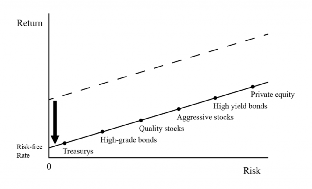
The diagram below illustrates:

Falling short-term interest rates reduce the yields of other asset classes

Conclusion

Government bond yields, a cornerstone of global financial markets, are influenced by a variety of interconnected factors.

At the heart of these determinants lies the intricate dance between monetary policy and broader economic conditions.

Monetary Policy

Central banks wield significant influence over bond yields through tools such as:

• Adjusting short-term interest rates.
• Implementing forward guidance, both outcome-based and time-based.
• Engaging in quantitative easing or asset buying.

The Taylor Rule

This framework, proposed by economist John Taylor, provides a mathematical approach to gauge the appropriate interest rate for an economy, factoring in inflation and output gaps.

Term Premia

This represents the extra compensation investors require for holding long-maturity bonds versus short-term debt.

It’s influenced by factors like inflation uncertainty, risk aversion, and changes in the demand for government bonds.

Non-Monetary Policy Drivers

Beyond central bank actions, bond yields are swayed by:

• Long-term growth and inflation expectations.
• Short-term business cycle fluctuations.
• The demand for liquid, safe-haven assets, especially during times of economic uncertainty.

Potential for Lower Yields

Factors such as central bank policies, economic downturns, low inflation expectations, and increased demand for safe assets can push bond yields even lower, as observed in some developed markets.

Summary

Government bond yields are not just mere numbers; they are a reflection of the broader economic landscape, central bank policies, market sentiment, and global events.

Understanding these determinants is important for traders, investors, policymakers, and anyone looking to keep tabs on the global economy.