Probability Distributions in Finance, Markets & Trading


Probability distributions are one of the most fundamental concepts in finance, markets, and trading.
They provide a fundamental framework for understanding, modeling, and managing the unknowns and risks inherent in these domains.
Trading isn’t so much about “predicting the future” (i.e., trying to ascertain a deterministic line of how things will transpire) as it is recognizing the probabilistic nature of the exercise, where future outcomes can be modeled as probability distributions.
The range of unknowns is high relative to the range of knowns relative to what’s discounted in the price.
A popular psychological bias, in general, is to naturally want to think in more deterministic ways with simple heuristics, rather than in more nuanced ways recognizing that a wide range of outcomes are possible.
Many things are possible, but with very different probabilities associated with them, which is the nature of probability distributions.
And in trading and markets, we tend to be biased by our own and recent experiences, and underweight the probability of “tail” events that are different from recent events.
Key Takeaways – Probability Distributions in Finance, Markets & Trading
- Modeling – Probability distributions are used to show the range of possible outcomes and estimated/discounted (or sometimes known) probabilities associated with each.
- Understand Risk – Probability distributions, especially tail behavior, are important for assessing market risks and extreme events.
- Optimize Portfolios – Moments like mean and variance are most fundamental. They’re commonly used for portfolio diversification and risk-return optimization.
- Pricing Derivatives – Higher-order moments (skewness, kurtosis) influence options pricing and implied volatility.
- Higher-order moments and cumulants allow for a more accurate and nuanced representation of the underlying asset’s expected return distribution.
- Their inclusion in pricing models helps to capture the risks associated with extreme market movements, which is critical for options. Options payoffs (in particular) can be highly sensitive to such movements.
- Identify Market Anomalies – Moments can reveal insights into market inefficiencies and trader/investor behavior.
- Informed Decision Making – Knowledge of distributions and moments helps in making more objective trading decisions.
- Conceptual Map for Understanding Moments
- Mean (1st Moment) – Central tendency or average level.
- Variance (2nd Moment) – Spread or average squared deviation from the mean.
- Skewness (3rd Moment) – Asymmetry or bias in one direction.
- Kurtosis (4th Moment) – Tailedness or the propensity for extreme values.
- Fifth Moment and Beyond – Increasingly complex aspects of the distribution’s shape, especially in the tails and extremities.
The Basics of Probability Distributions in Finance, Markets & Trading
Probability distributions in finance, markets, and trading are mathematical functions that represent the likelihood of different outcomes or returns on an investment or trade.
This helps in risk assessment and decision-making by quantifying unknowns and potential variations in market behaviors or financial asset performances.
Probability Distributions & Time Evolution
The time evolution nature of probability distributions in finance reflects that as time progresses, the range and shape of potential outcomes for asset returns or market behaviors can shift, indicating changing risks, potential outcomes, and unknowns.
This necessitates dynamic and ongoing adjustments in risk assessment and trading/investment strategies.
Non-Finance Example
Say you were plotting out the height and weight ranges for people based on their age, gender, location, and other data.
For example, if you wanted to predict the height of an American male, you know he’s more likely to be 6 feet than 7 feet or 5 feet, and his weight is more likely to be 200 lbs than 300 lbs or 100 lbs.
But he could be anywhere within that range (or even outside of that range), but with highly varying probabilities within a wide set of possibilities.
And there’s also the nature of the distribution.
- Are outliers more common (do we have wider tails, or more kurtosis)?
- What is the skew of the distribution? If the mean is 5’10”, is the population evenly distributed on each side or are taller or shorter people more common? And so on.
- What are the variables that influence the distribution?
- How does the distribution change over time?
- How is it different for other regions, sub-regions, or other demographics?
If there was a market where betting on this was possible, we would need to collect as much information as we could do to plot out the nature of the distribution, compare that to the market-discounted distribution (based on actual bets made within the relevant markets), and use that to make our own bets (if possible) that provide positive expected value.
Here’s a basic overview of the importance of probability distributions across various categories:
Risk Assessment and Management
Understanding Asset Returns
Probability distributions help in modeling the returns of different financial assets.
By understanding the distribution of returns, traders can better know the risk and potential rewards associated with an asset.
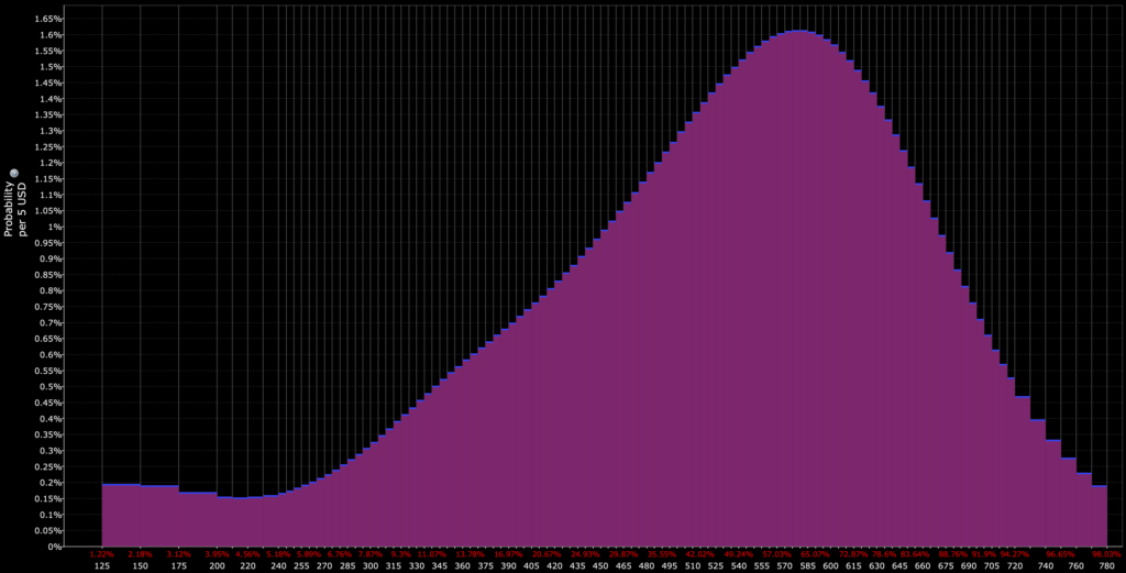
For example, if we wanted a probability distribution of the return of SPY more than two years forward, we see a wide distribution of potential outcomes:
Tail Risk
Distributions with heavy tails highlight the potential for extreme events (“black swan” events) or simply events that would occur more than you might think.
This helps in preparing for unlikely but potentially devastating market movements.
Portfolio Construction
Diversification
By understanding the joint distributions of asset returns, traders/investors can construct portfolios that optimize the risk-return trade-off.
Correlation and Covariances
This involves assessing correlations and covariances, which are derived from the joint probability distributions of asset returns OR by understanding what they’re fundamentally like and not simply going based on past data (that may not represent the future).
Efficient Frontier
The concept of the efficient frontier in portfolio theory, which represents the set of optimal portfolios offering the maximum possible expected return for a given level of risk, is based on the probability distribution of returns.
In modern quantitative finance, mean-variance optimization is an overly simplistic framework, but the general idea (being compensated for risk, diversification to improve risk-adjusted returns) holds true.
Many common risk-adjusted return metrics are based on the first two moments of the distribution or variations of it (e.g., Sharpe, Sortino).
Derivative Pricing
Options Pricing Models
Models like Black-Scholes use probability distributions (typically normal or log-normal) to price options.
These models incorporate the distribution of potential future prices of the underlying asset to calculate the fair value of options.
Implied Volatility
The concept of implied volatility, which is a huge component in options pricing, is derived from the market’s consensus view of the future distribution of asset prices.
Market Behavior Analysis
Behavioral Finance
Probability distributions are used to study market anomalies and trader/investor behavior.
For instance, distributions that capture skewness and kurtosis can explain why investors might have preferences for assets with “lottery-like” (convex) payoffs.
Market Prediction Models
Statistical models and machine learning algorithms often rely on probability distributions to predict market movements and identify trading opportunities.
Risk-Adjusted Performance Measurement & Algorithmic Trading
Performance Metrics
Metrics like the Sharpe ratio, Sortino ratio, and Value at Risk (VaR) rely on the distribution of asset returns to measure the risk-adjusted performance of trades or investments.
Stress Testing
Financial institutions use probability distributions in stress testing and scenario analysis to evaluate how portfolios would perform under various adverse market conditions.
Quantitative Strategies
Many algorithmic trading strategies are based on statistical models that assume specific probability distributions for asset prices and returns – or at least use these functional forms for prototyping algorithms in development.
For example, in a lot of our articles, we generally prototype in Python using normal distributions when showing a conceptual example.
Mathematical models are used to identify patterns and execute trades.
Risk Control
Algorithmic trading also uses probability distributions to set risk limits and parameters.
This ensures that automated trading strategies operate within acceptable risk confines.
Mean & Variance
In probability distributions, the mean and variance are two fundamental concepts that describe key characteristics of the distribution.
Mean
The mean, often referred to as the expected value or average, is a measure of the central tendency of a distribution.
It’s calculated as the sum of all possible values weighted by their respective probabilities.
In simple terms, it represents the average outcome if an experiment or process were repeated many times.
For instance, in a dice roll, the mean value is 3.5, representing the average outcome of rolling the dice repeatedly.
Also, in a closed system like throwing two dice, we know the probability distribution associated with this.
Variance
The variance measures the spread or dispersion of the distribution around the mean.
It’s calculated as the average of the squared differences from the mean, providing a sense of how much individual values in the distribution deviate from the mean.
A high variance indicates that the data points are spread out over a wider range of values, while a low variance indicates that they are clustered closely around the mean.
For example, in a distribution where all values are identical, the variance is zero, as there is no deviation from the mean.
Together, the mean and variance provide a basic but usually strong description of the behavior of a probability distribution by indicating both its central tendency and the variability of outcomes.
Similar Terms to Mean and Variance
Many analogous terms in finance are used interchangeably or near-interchangeably with mean and variance.
Examples include return (mean) and volatility or risk (variance).
Skew & Kurtosis
Skew and kurtosis are “higher moments” used to describe a probability distribution.
Skew
Skewness in finance refers to the asymmetry in the distribution of asset returns.
It indicates a tendency for returns to lean more toward one side of the mean.
A positive skew implies more frequent small losses and occasional large gains, while a negative skew indicates frequent small gains and rare large losses.
Kurtosis
Kurtosis measures the “tailedness” of the return distribution.
High kurtosis suggests a higher probability of extreme returns (either very high or very low) compared to a normal distribution.
This increases the potential risk and unpredictability of an investment.
Optimizing Skew and Kurtosis
Beyond optimizing for mean (as high as possible) and variance (as low as possible), to optimize for skew and kurtosis, we want skew as positive as possible (greater chance for high returns) and kurtosis low (to minimize tail risks).
For example, if we revisit the distribution from earlier in the article, this has positive skew and high kurtosis.
These types of characteristics make sense, as this is SPY (ETF of the S&P 500 index), where stocks have positive expected return (positive “drift”) and fatter tails relative to what a normal distribution would predict.
The normal distribution is characterized by zero skew and zero kurtosis.
Skew and Tailedness Example: Natural Gas
This probability distribution of natural gas (the UNG ETF) illustrates a fundamental concept in commodity pricing: the difference between the most likely outcome and the market’s implied “fair value.”
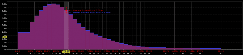
The distribution shows natural gas price probabilities for a particular expiry using UNG options data, showing an asymmetric pattern typical of commodity markets.
The purple area represents the probability distribution, with the y-axis showing probability percentages and the x-axis showing price levels.
Notice how the distribution has a distinctive shape – it peaks around $12-13 (where probabilities are highest at roughly 6%), but then has a long “tail” extending to the right toward much higher prices.
This asymmetric shape occurs because natural gas prices have limited downside (production costs as a type of floor, though not strictly) but theoretically unlimited upside during supply disruptions, geopolitical events, or extreme weather.
A pipeline explosion, war, or brutal winter could send prices a lot higher, creating those low-probability but high-impact scenarios in the right tail.
The key insight is that while the market-implied probability of the $16-17 level (shown in blue) sits around 5.59%, the highest probability outcomes cluster below this level.
This means the market is pricing in a premium for those tail risks – i.e., the small chance of extreme price spikes pulls the average expected price higher than the most likely individual outcomes.
This pattern explains why natural gas markets often seem “expensive” relative to base-case scenarios.
The market isn’t just pricing the most probable outcome, but incorporating the weighted average of all possible outcomes, including those low-probability but extreme price scenarios.
For traders, this highlights why commodity investments can be challenging – you’re not just betting on the most likely scenario, but on whether the market has properly priced the full range of possibilities, including those fat-tail risks that can dramatically impact returns.
Higher-Order Moments & Other Concepts in Probability Distributions
In financial probability distributions, moments beyond the ones we referenced (mean, variance, skewness, and kurtosis) become increasingly complex and abstract.
Nevertheless, they can provide deeper insights into the behavior of financial variables.
Here are some additional moments and related concepts:
Higher-Order Moments
These include the 5th, 6th, and higher moments of a distribution.
While their practical interpretation is less intuitive than the first four moments, they can capture more detailed aspects of the distribution’s shape – particularly in the tails.
Cumulants
Cumulants are related to moments but have certain advantageous properties.
The first four cumulants are identical to the first four moments (mean, variance, skewness, kurtosis).
But higher-order cumulants can offer different insights into the structure of the distribution, mostly in terms of dependencies and relationships between variables.
Central Moments
These are moments about the mean of the distribution.
While the first central moment is always zero, higher central moments can provide information about the distribution’s shape relative to its mean.
L-Moments
L-moments are linear combinations of order statistics.
They’re useful in the analysis of data with heavy tails or outliers.
L-moments are often used for more robust estimation of distribution parameters than conventional moments.
Moment Generating Functions
While technically not a moment, the moment-generating function (MGF) of a distribution can be used to find all the moments of the distribution.
The nth derivative of the MGF, evaluated at zero, gives the nth moment.
Characteristic Function
Similar to the MGF, the characteristic function can be used to derive all moments of a probability distribution.
It’s useful for distributions where there’s no MGF.
Entropy
In the context of information theory, entropy measures the uncertainty or randomness of a distribution.
It’s not a moment in the traditional sense but provides a different perspective on the distribution’s characteristics.
Co-skewness and Co-kurtosis
These are measures of how one random variable changes in relation to the skewness and kurtosis of another random variable.
They’re important in portfolio theory for understanding the joint behavior of asset returns.
Tail Dependence
While not a moment, tail dependence is a concept in financial risk management.
It measures the likelihood of extreme movements in one variable occurring simultaneously with extreme movements in another.
Conditional Moments
These are moments calculated under certain conditions or assumptions. Conditional variance is a key concept in volatility modeling.
Official Moments
Labeling and conceptualizing higher-order moments beyond the fourth moment (kurtosis) can be challenging, as their practical interpretations are less intuitive and more abstract.
But we can still label them and provide a generalized map to conceptualize these moments:
First Moment – Mean
This is the average value of the distribution.
It provides the central location or the expected value of the distribution.
Second Moment – Variance
This measures the dispersion or spread of the distribution around the mean.
It’s a measure of the distribution’s width and gives an idea of how much individual values typically deviate from the mean.
Third Moment – Skewness
Skewness indicates the asymmetry of the distribution.
A positive skew means a longer or fatter tail on the right side.
A negative skew means a longer or fatter tail on the left.
Fourth Moment – Kurtosis
This measures the “tailedness” of the distribution.
High kurtosis indicates heavy tails and a sharp peak (leptokurtic).
Low kurtosis indicates light tails and a flat peak (platykurtic).
Fifth Moment and Beyond
Higher-order moments (5th, 6th, etc.) continue to describe increasingly complex and subtle characteristics of the distribution’s shape, mostly in the tails.
Fifth Moment
Measures the asymmetry of the tails.
Unlike skewness, which measures asymmetry in one direction, the fifth moment captures it in a more complex way.
Sixth Moment and Higher
These moments capture increasingly fine details about the distribution’s shape, particularly extremities and oddities in the tails.
Applications of 5th Order Moments and Beyond
The first four moments have clear and widely accepted interpretations, but higher moments become progressively more abstract and less intuitive.
In financial analysis, moments beyond the fourth are rarely used due to the difficulty in their estimation and interpretation.
Their practical utility often lies in specific theoretical contexts or in advanced statistical and quantitative modeling.
Cumulants
Discussing higher-order cumulants involves going into more complex aspects of statistical distribution characterization.
Cumulants, like moments, are a set of statistics that describe various features of a probability distribution.
While the first and second cumulants correspond to the mean and variance, respectively, higher-order cumulants offer a deeper understanding of the distribution’s shape, particularly its asymmetry and tail behavior.
Higher-Order Cumulants
Third Cumulant (Equivalent to Skewness)
- Describes the asymmetry of a distribution.
- A positive third cumulant indicates a distribution with a longer or heavier tail on the right side, while a negative value indicates a longer or heavier tail on the left.
- In finance, positive skewness is often preferred as it suggests a higher likelihood of extreme positive returns.
Fourth Cumulant (Excess Kurtosis)
- Measures the “tailedness” or the propensity for extreme outcomes in a distribution.
- A higher fourth cumulant indicates a distribution with heavier tails and a sharper peak compared to a normal distribution.
- In financial terms, high kurtosis implies a higher risk of extreme market moves, both up and down.
Fifth Cumulant and Beyond
- These cumulants capture increasingly complex aspects of the distribution’s shape in the tails.
- The fifth cumulant can provide insights into the asymmetry of the tails, different from the skewness captured by the third cumulant.
- Higher cumulants (sixth, seventh, etc.) are more challenging to interpret and are less commonly used, but they continue to describe finer and more subtle characteristics of the distribution (like nuances in the shape of its tails).
Significance in Probability and Finance
Probability Theory
In probability theory, higher-order cumulants are important for understanding the detailed structure of probability distributions, especially in the context of advanced statistical modeling and theoretical studies.
While the first few cumulants (mean, variance, skewness, kurtosis) are widely used and understood, higher-order cumulants have a more specialized role in statistics and finance (mostly in situations where tail risk and extreme events are of particular concern).
Finance
In finance, higher-order cumulants are highly relevant in the areas of risk management and derivative pricing.
They provide information about the likelihood and impact of extreme market movements, which is important for pricing options and other financial derivatives.
For instance, options pricing models, such as those used in the valuation of exotic options, may require an understanding of higher-order cumulants to accurately capture the risk of large market moves.
Other quants might study higher-order moments/cumulants to gain a trading edge in some way.
Practical Challenges
Higher-order cumulants become increasingly difficult to estimate accurately from empirical data.
Therefore, their practical usage is often limited to theoretical studies or specific contexts where the precise characterization of distribution tails is essential.
Moments vs. Cumulants
Moments and cumulants are two different but related ways of describing the characteristics of a probability distribution.
Moments provide a direct and intuitive way to understand the characteristics of a distribution.
Cumulants offer a more nuanced view, especially for the analysis of tail risks and extreme events in finance.
Moments are generally more commonly used for basic financial analysis, but cumulants become important in more complex quantitative finance areas.
Understanding them in the context of finance can be quite insightful, particularly when analyzing risk and return profiles of assets/investments/instruments/trades.
Here’s a simple explanation (and a little bit of review from above):
Moments
What They Are
Moments are quantitative measures related to the shape of a distribution’s probability density function.
They include mean (first moment), variance (second moment), skewness (third moment), and kurtosis (fourth moment), among others.
Types
The first moment is the mean, the second is the variance (spread of the distribution), the third is skewness (asymmetry), and the fourth is kurtosis (tailedness).
In Finance
Moments are useful in assessing investment risks and returns.
For example, the mean (first moment) indicates the expected return of a financial asset, while the variance (second moment) measures the asset’s volatility or risk.
Skewness (third moment) and kurtosis (fourth moment) are important when considering the likelihood of extreme returns or “black swan” events.
Cumulants
What They Are
Cumulants, like moments, provide a way to describe a distribution, but they focus more on the distribution’s structure in terms of central peak and tails.
Cumulants are derived from the logarithm of the characteristic function of a distribution, where the first few cumulants correspond to the mean, variance, skewness, and kurtosis, but differ in higher orders and provide a more nuanced description of distribution characteristics.
Relation to Moments
The first and second cumulants are the same as the first two moments (mean and variance).
The higher cumulants (third, fourth, etc.) aren’t as precisely equal as the corresponding moments but provide additional insights into the distribution’s shape.
In Finance
Cumulants, particularly the higher-order ones, can be helpful in financial modeling and risk assessment, especially in complex derivative pricing and risk modeling.
They may offer a more nuanced understanding of the distribution’s tail behavior for purposes of risk management.
Examples and Relation to Probability and Finance
- Mean (1st Moment) / 1st Cumulant – This represents the average return of a financial asset. For instance, if a stock has an average annual return of 8%, the mean or first moment/cumulant of its return distribution is 8%.
- Variance (2nd Moment) / 2nd Cumulant – This measures the variability or risk of the asset’s returns. A higher variance indicates greater risk. If a stock’s returns vary greatly from year to year, it has a high variance.
- Skewness (3rd Moment) – In finance, skewness can indicate the tendency of an asset to have asymmetric returns. Positive skewness might imply a greater likelihood of exceptionally high returns, while negative skewness suggests a higher risk of substantial losses.
- Kurtosis (4th Moment) – High kurtosis in a financial asset suggests a higher risk of extreme returns (both positive and negative). For instance, stocks often have high kurtosis due to their potential for both very high gains and substantial losses.
- Higher-Order Cumulants – These become important in advanced financial models, such as those used in options pricing, where the tail behavior of the asset returns can significantly impact the valuation of financial derivatives.
Cumulants for Parametric vs. Non-Parametric Data
Cumulants, including higher-order ones, can be used to characterize both parametric and non-parametric distributions.
Their application isn’t limited to distributions with specific parameters.
This makes them versatile tools in statistical analysis and practical/real-world applications.
Parametric Distributions
Parametric distributions are those that are fully described by a set of parameters.
Classic examples include the normal distribution, binomial distribution, and Poisson distribution.
Cumulants in Parametric Distributions
For these distributions, cumulants can often be explicitly calculated based on the distribution’s parameters.
For instance, in a normal distribution, all cumulants beyond the second are zero, which is a distinctive property of the normal distribution.
Non-Parametric Distributions
Non-parametric distributions don’t assume a specific functional form.
They’re often used when there is little prior knowledge about the distribution shape or when the data doesn’t fit well into common parametric forms.
Cumulants in Non-Parametric Distributions
Cumulants can be estimated from the data without assuming any specific distribution model.
This makes them useful in real-world applications where the underlying probability distribution is unknown or complex.
Applications
In finance, for example, asset return distributions are often non-parametric, with characteristics like skewness and heavy tails that are not well-captured by simple parametric models.
Cumulants can provide a deeper understanding of such distributions, which is important for risk management and derivative pricing.
Practical Considerations
Estimation Challenges
Estimating higher-order cumulants in non-parametric distributions can be challenging.
This is especially true from limited sample sizes, as these estimates can become increasingly sensitive to sampling error.
Interpretation
The first four cumulants (mean, variance, skewness, and kurtosis) have clear interpretations, higher-order cumulants can be more difficult to interpret – particularly in the context of non-parametric models.
Higher-Order Moments & Cumulants in the Context of Options Pricing
In the context of options pricing, higher-order moments and cumulants capture the nuances of asset return distributions, which can have profound implications on the valuation of options.
Options are sensitive not just to the mean and variance of the underlying asset’s returns (as captured by the first two moments/cumulants) but also to the shape of the return distribution, which is where higher-order moments and cumulants become important.
Higher-Order Moments in Options Pricing
Skewness (3rd Moment)
- Role – Skewness affects how asymmetric the return distribution is, which influences the pricing of out-of-the-money (OTM) options.
- Impact – Positive skewness indicates a higher probability of extreme positive returns, which might increase the price of OTM calls. Conversely, negative skewness, indicating a higher probability of extreme negative returns, can increase the price of OTM puts.
Kurtosis (4th Moment)
- Role – Kurtosis measures the “fatness” of the tails of the distribution. High kurtosis implies a higher probability of extreme returns, both positive and negative.
- Impact – Higher kurtosis increases the value of both OTM calls and puts, as it suggests a greater likelihood of significant price movements, either upward or downward.
Higher-Order Cumulants in Options Pricing
Third and Fourth Cumulants
- These are closely related to skewness and kurtosis, respectively, and influence options pricing similarly by affecting the valuation of OTM options.
- In advanced options pricing models, such as those used for exotic options, the precise characterization of the return distribution’s tail behavior (as described by higher-order cumulants) can be very important.
Practical Application
Standard Models
Traditional models like the Black-Scholes model assume a normal distribution of returns (i.e., no skewness or excess kurtosis).
Unfortunately, this assumption often fails to capture the reality of financial markets, where skew and fat tails are the norm.
Advanced Models
To address this, more sophisticated models – e.g., stochastic volatility models or jump-diffusion models – incorporate these higher-order moments.
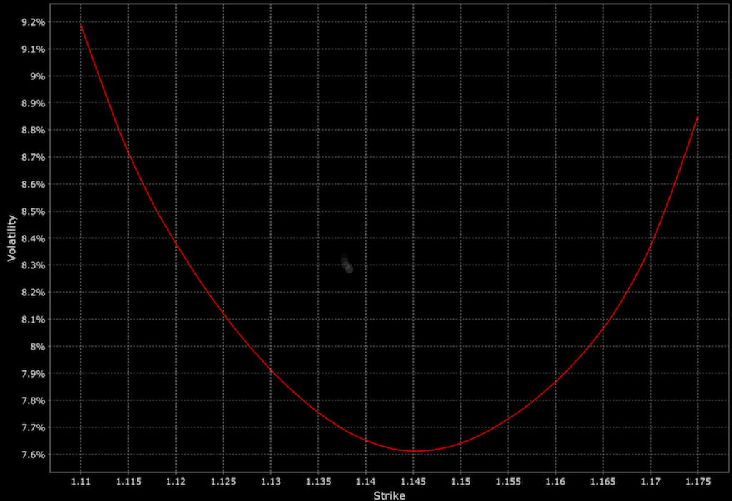
These models are better equipped to handle real-world financial markets, like sudden jumps in prices or the volatility smile – a pattern observed in the implied volatility of options across different strike prices.
Implications
The incorporation of higher-order moments and cumulants allows for more accurate pricing of options – notably in situations where extreme market moves are more probable or during periods of market stress.
(Options are convex instruments and much more sensitive to extreme movements than the underlying asset.)
Conclusion: Understand That Markets Are Probabilistic
Markets are probabilistic because they are made up of a vast number of transactions, each of which is a simple exchange between a buyer and a seller.
When you look at any market, you’re seeing the sum of all these transactions. If you know how much money and credit is being spent and how much of each item or asset is being sold, you understand the market.
The probabilistic nature of markets comes into play when we try to predict what will happen next.
We can’t predict with certainty what each buyer and seller will do, but we can make educated guesses based on past behavior, economic trends, and other factors.
So, we talk about probabilities and the distribution of likelihood of these various possibilities – what’s more or less likely to happen, not what will definitely happen.
For example, if a company is reporting strong earnings and the economy is doing well, it’s likely that the company’s stock price will go up. But there’s no guarantee.
Everything that’s known is baked in the price.
That’s why trading and investing always involves risk, and that’s why it’s important to diversely trade or invest and not put all your eggs in one basket.
But Don’t Overwhelm Yourself
When you’re trying to make a decision, especially in trading or investing, you want to have as much information as possible.
But there’s a point where getting more information doesn’t help you make a better decision. In fact, it can even make things worse by confusing you or causing you to doubt what you already know.
Think of it like this: if you’re trying to decide whether to bring an umbrella when you go out, you might look at the weather forecast.
If the forecast says there’s a 40% chance of rain, you might decide to bring an umbrella because the downside of it raining makes it too risky not to bring one.
But if you start looking at more and more forecasts, and they all say different things, you might end up more confused than when you started. You might even decide not to bring an umbrella, even though the first forecast was probably reasonably accurate.
The same thing can happen with trading. If you do too much research, you might end up with so many different opinions and predictions that you don’t know what to do.
You might even end up making a worse decision than if you had just stuck with what you knew initially.
So, it’s important to weigh the value of additional information against the cost of not deciding. Sometimes, it’s better to make a decision with the information you have than to keep searching for more information and risk making a worse decision.
In other words, don’t let the search for perfect information prevent you from making good decisions.
Always be sure to think carefully about how you decide when you have enough information to make a decision.
Article Sources
- https://www.cell.com/heliyon/pdf/S2405-8440(22)00121-9.pdf
- https://www.sciencedirect.com/science/article/pii/S0140988323000944
- https://www.sciencedirect.com/science/article/pii/S0927539814000966
The writing and editorial team at DayTrading.com use credible sources to support their work. These include government agencies, white papers, research institutes, and engagement with industry professionals. Content is written free from bias and is fact-checked where appropriate. Learn more about why you can trust DayTrading.com