Mean-Variance Optimization

Mean-Variance Optimization, also known as the Two-Moment Decision Model, is a popular financial metric developed by Harry Markowitz in 1952.

It forms the basis for modern portfolio theory and assists in the construction of investment portfolios.

This analysis hinges on two key statistical measures:

• the mean, representing expected returns, and
• the variance, indicating risk or volatility

Key Takeaways – Mean-Variance Optimization

• Risk-Return Trade-Off
  • Mean-Variance Optimization balances the trade-off between risk and return.
  • Aims for the highest return for a given level of risk.
• Diversification
  • By considering correlation and covariance, it effectively diversifies portfolio allocation.
• Efficient Frontier
  • It identifies the set of optimal portfolios that offer the highest expected return for a defined level of risk, known as the efficient frontier.
  • We do a coding example of mean-variance optimization and the efficient frontier diagram below.

Core Principles

Expected Returns (Mean)

The mean in this context is the average expected return of an investment portfolio – a central measure to estimate the future performance of the portfolio.

It’s calculated based on the weighted average of the expected returns of individual assets in the portfolio.

Risk Measurement (Variance)

Variance, the second element, quantifies the dispersion of returns around the mean.

In financial terms, it represents the degree of risk associated with the investment portfolio.

A higher variance implies greater volatility, indicating a higher risk level.

Application in Portfolio Optimization

Diversification and Efficient Frontier

Mean-variance optimization is used in achieving portfolio diversification.

It aids in selecting a mix of assets that minimizes risk for a given level of expected return.

The concept of the “Efficient Frontier” emerges from this analysis – a set of optimal portfolios offering the highest expected return for a defined level of risk.

We’ll look at an example below.

Asset Allocation

This analysis guides traders in asset allocation.

By understanding the risk-return trade-off, traders can allocate their resources to various assets in a manner that aligns with their risk tolerance and investment goals.

Example of Mean-Variance Optimization

Here’s our Python code, where we design an optimized portfolio between stocks and bonds.

We make these example assumptions:

• Stocks: 7% returns, 15% vol
• Bonds: 5% returns, 10% vol
• 0% long-run correlation

We’ll describe what the results were after giving the code.

import numpy as np
import pandas as pd
import matplotlib.pyplot as plt
from scipy.optimize import minimize

# Random seed
np.random.seed(76)

# Asset details for the new scenario
assets = ['Stocks', 'Bonds']
returns_annual = np.array([0.07, 0.05])
volatility_annual = np.array([0.15, 0.10])
correlation_matrix = np.array([[1.0, 0.0], # 0% correlation between stocks and bonds
[0.0, 1.0]])

# Generate covariance matrix from volatilities and correlation matrix
covariance_matrix = np.outer(volatility_annual, volatility_annual) * correlation_matrix

# Number of portfolios to sim
num_portfolios = 10000

# Simulate random portfolio weights
np.random.seed(76)
weights_record = []
returns_record = []
volatility_record = []
for _ in range(num_portfolios):
weights = np.random.random(len(assets))
weights /= np.sum(weights)
weights_record.append(weights)

# Expected portfolio return
returns = np.dot(weights, returns_annual)
returns_record.append(returns)

# Expected portfolio volatility
volatility = np.sqrt(np.dot(weights.T, np.dot(covariance_matrix, weights)))
volatility_record.append(volatility)

weights_record = np.array(weights_record)
returns_record = np.array(returns_record)
volatility_record = np.array(volatility_record)

# Plotting the new portfolios
plt.scatter(volatility_record, returns_record, c=returns_record/volatility_record, cmap='YlGnBu', marker='o')
plt.title('Simulated Portfolios')
plt.xlabel('Expected Volatility')
plt.ylabel('Expected Return')
plt.colorbar(label='Sharpe Ratio')
plt.show()

# Function to calculate the negative Sharpe ratio
def negative_sharpe(weights, returns, covariance):
portfolio_return = np.dot(weights, returns)
portfolio_vol = np.sqrt(np.dot(weights.T, np.dot(covariance, weights)))
return -portfolio_return / portfolio_vol

# Constraints and bounds
constraints = ({'type': 'eq', 'fun': lambda x: np.sum(x) - 1}) # The sum of weights is 1
bounds = tuple((0, 1) for asset in range(len(assets)))

# Initial guess (equal distribution)
init_guess = np.array([1. / len(assets) for asset in assets])

# Optimize for the new scenario
optimal_sharpe = minimize(negative_sharpe, init_guess, args=(returns_annual, covariance_matrix),
method='SLSQP', bounds=bounds, constraints=constraints)

# Results for the new scenario
optimal_weights = optimal_sharpe.x
optimal_return = np.dot(optimal_weights, returns_annual)
optimal_volatility = np.sqrt(np.dot(optimal_weights.T, np.dot(covariance_matrix, optimal_weights)))

optimal_weights, optimal_return, optimal_volatility

(If using this code, please be sure to indent where appropriate given this is Python.)

The Python model for mean-variance optimization is modeled based on an efficient frontier diagram that shows the mean-variance trade-off:

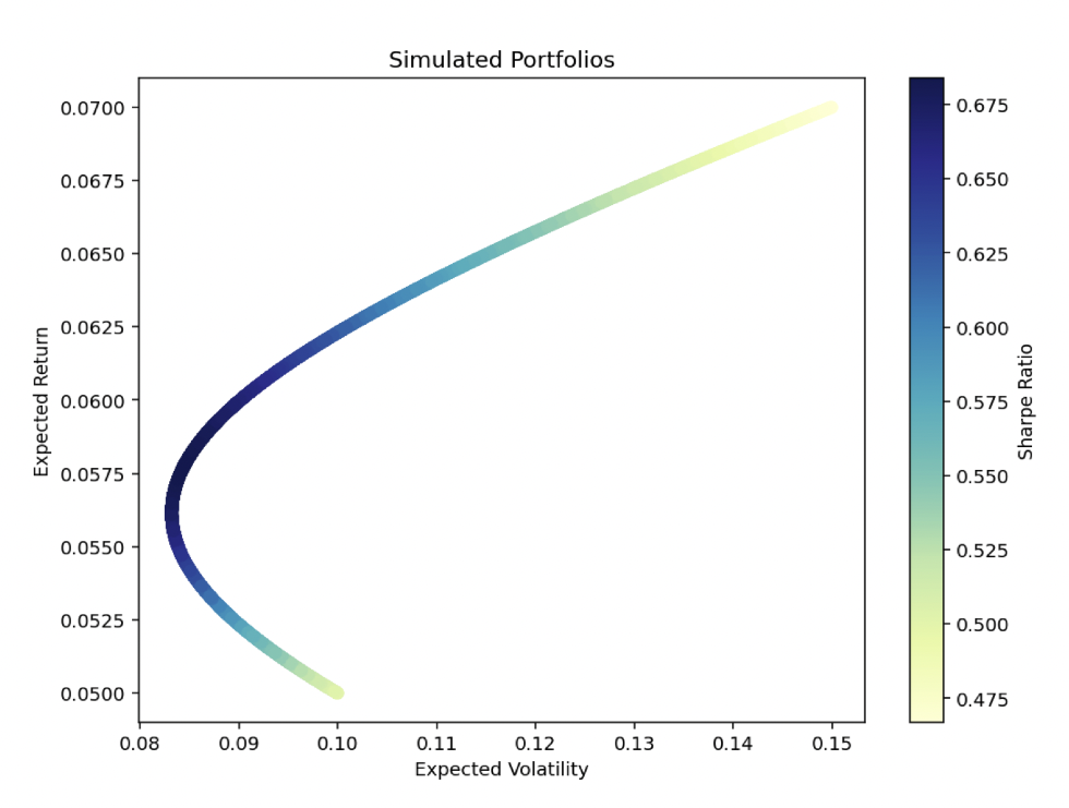
For the scenario with 7% expected returns and 15% volatility for stocks, and 5% expected returns and 10% volatility for bonds with 0% correlation, the mean-variance optimization model yields:

• Optimal Weights:
  • Stocks: 38.37%
  • Bonds: 61.63%
• Optimal Portfolio Expected Return: 5.77%
• Optimal Portfolio Expected Volatility: 8.43%

This optimal portfolio allocation is designed to maximize the Sharpe ratio, balancing the trade-off between expected returns and volatility.

The allocation slightly favors bonds over stocks, reflecting the different return and risk profiles of the assets and the goal of achieving a balance between risk and return in the portfolio.

The expected annual return is approximately 5.77% with a volatility of 8.43%.

This shows how basic diversification can improve the return-to-risk ratio significantly.

Instead of getting only about 0.47-0.50% of return for each percentage point in volatility, it moves up to 0.68% of return per percentage point in volatility.

Limitations and Considerations

Assumptions & Real-World Application

Mean-variance optimization assumes normally distributed returns and constant variance over time.

It also ignores “higher moments” that describe the shape of expected distributions of returns – i.e., skewness and kurtosis.

In real-world scenarios, these assumptions may not hold true, potentially leading to deviations in actual portfolio performance.

Time Horizon and Risk Preferences

The effectiveness of this model also depends on the trader/investor’s time horizon and risk preferences.

Short-term day traders might find the model less applicable due to its reliance on long-term averages and tendencies.

Conclusion

Mean-variance optimization remains foundational in finance for portfolio construction and management.

Despite its limitations and assumptions, it provides a structured approach to understanding the trade-off between risk and return.