Correlation vs. Covariance in Asset Allocation

Correlation and covariance are statistical measures in asset allocation.

They provide information on how different financial assets move in relation to each other.

Covariance measures the directional relationship between the returns of two assets.

When the covariance is positive, asset returns move together; if negative, they move inversely.

Correlation, meanwhile, standardizes this relationship, expressing it on a scale from -1 to 1.

A correlation of 1 indicates perfect positive movement, -1 signifies perfect inverse movement, and 0 represents no linear relationship.

Key Takeaways – Correlation vs. Covariance in Asset Allocation

• Covariance indicates direction of returns: It shows whether assets move together but doesn’t account for the scale.
• Correlation standardizes covariance: Providing a scaled measure (-1 to 1) showing the strength and direction of the relationship.
• Both are important in diversification: Helping to minimize risk and maximize return through informed asset allocation.
• Coding example: We run a coding example to show how to optimize a portfolio using correlation, covariance, and other important information, along with an efficient frontier diagram.

Application in Diversification Strategies

In asset allocation, understanding these metrics is important for diversification.

Diversification aims to reduce risk by combining assets with varying correlations.

A portfolio with assets having low or negative correlations can withstand market fluctuations better.

In this article, we explained how the lower the correlation the better the improvement in the return-to-risk ratio (assuming positive expected returns in the returns streams).

Past Correlations Aren’t Indicative of Future Correlations

Correlations between assets like stocks and bonds should not be inferred solely from past behavior but rather from their intrinsic characteristics.

For instance, stocks and bonds are typically negatively correlated. This intrinsic relationship largely manifests when changes in discounted growth rates primarily influence their prices.

Stocks generally flourish in high growth environments, while bonds perform better when growth is slow, reflecting their inverse relationship.

However, this correlation can reverse under different economic conditions, such as when changes in discounted inflation become the dominant factor affecting prices.

In such scenarios, both stocks and bonds might react similarly to inflationary trends, thus exhibiting a positive correlation.

Intrinsic Nature of Assets > Past Correlations

Accordingly, the intrinsic nature of assets, governed by their fundamental economic underpinnings, should be the primary focus when assessing correlation, rather than relying exclusively on historical data.

Correlations looking in the rear-view mirror are fleeting byproducts of their behavior in a particular environment.

This approach acknowledges that correlations are dynamic and subject to change based on the prevailing economic forces at play.

Traders/Investors Learning Also Impact Future Data

Traders/investors also learn new things about how markets and economies work over time.

This learning has the effect of changing future data relative to how things may have worked in the past.

This is another danger of using past correlations to inform how to trade going forward.

Impact on Portfolio Risk Management

Covariance and correlation are instrumental in modern portfolio theory (MPT), a framework introduced by Harry Markowitz in 1952.

MPT suggests that an optimal portfolio is one that offers the highest expected return for a given level of risk – mean-variance optimization.

This risk is assessed through the covariance matrix of the asset returns.

Correlation coefficients further assist in identifying the diversification benefits.

For example, during the 2008 financial crisis, some asset correlations (particularly those within the same asset class or in similar risky asset classes) converged towards 1, indicating a failure in traditional diversification strategies.

This observation led to the increased use of alternative assets (including liquid alternatives) to achieve true diversification.

Quantitative Analysis in Asset Selection

Quantitative analysts use these statistics to construct efficient frontiers – graphs showing the optimal portfolio mix.

By calculating the expected returns, variances, and covariances of different assets, they identify portfolios offering the maximum return for a given risk level.

Correlation vs. Covariance in Asset Allocation – Coding Example

Here’s our Python code, where we design an optimized portfolio between stocks and bonds.

We make these assumptions:

• Stocks: 6% returns, 15% vol
• Bonds: 4% returns, 10% vol
• 0% long-run correlation

We’ll describe what the results were after giving the code.

import numpy as np
import pandas as pd
import matplotlib.pyplot as plt
from scipy.optimize import minimize

# Set random seed
np.random.seed(96)

# Asset details
assets = ['Stocks', 'Bonds']
returns_annual = np.array([0.06, 0.04])
volatility_annual = np.array([0.15, 0.10])
correlation_matrix = np.array([[1.0, 0.0],
[0.0, 1.0]])

# Generate covariance matrix from volatilities and correlation matrix
covariance_matrix = np.outer(volatility_annual, volatility_annual) * correlation_matrix

# Number of portfolios to simulate
num_portfolios = 10000

# Simulate random portfolio weights
np.random.seed(96)
weights_record = []
returns_record = []
volatility_record = []
for _ in range(num_portfolios):
weights = np.random.random(len(assets))
weights /= np.sum(weights)
weights_record.append(weights)

# Expected portfolio return
returns = np.dot(weights, returns_annual)
returns_record.append(returns)

# Expected portfolio volatility
volatility = np.sqrt(np.dot(weights.T, np.dot(covariance_matrix, weights)))
volatility_record.append(volatility)

weights_record = np.array(weights_record)
returns_record = np.array(returns_record)
volatility_record = np.array(volatility_record)

# Convert lists of returns and volatilities to arrays for plotting
returns_record = np.array(returns_record)
volatility_record = np.array(volatility_record)

# Plotting the portfolios
plt.scatter(volatility_record, returns_record, c=returns_record/volatility_record, cmap='YlGnBu', marker='o')
plt.title('Simulated Portfolios')
plt.xlabel('Expected Volatility')
plt.ylabel('Expected Return')
plt.colorbar(label='Sharpe Ratio')
plt.show()

# Mean-Variance Optimization (Efficient Frontier)

# Function to calculate the negative Sharpe ratio (since we minimize the negative Sharpe in optimization)
def negative_sharpe(weights, returns, covariance):
portfolio_return = np.dot(weights, returns)
portfolio_vol = np.sqrt(np.dot(weights.T, np.dot(covariance, weights)))
return -portfolio_return / portfolio_vol

# Constraints
constraints = ({'type': 'eq', 'fun': lambda x: np.sum(x) - 1}) # The sum of weights is 1
bounds = tuple((0, 1) for asset in range(len(assets)))

# Initial guess (equal distribution)
init_guess = np.array([1. / len(assets) for asset in assets])

# Optimize
optimal_sharpe = minimize(negative_sharpe, init_guess, args=(returns_annual, covariance_matrix),
method='SLSQP', bounds=bounds, constraints=constraints)

# Results
optimal_weights = optimal_sharpe.x
optimal_return = np.dot(optimal_weights, returns_annual)
optimal_volatility = np.sqrt(np.dot(optimal_weights.T, np.dot(covariance_matrix, optimal_weights)))

optimal_weights, optimal_return, optimal_volatility

(If using this code, please be sure to indent where appropriate given this is Python.)

• Optimal Weights:
  • Stocks: 40.05%
  • Bonds: 59.95%
• Optimal Portfolio Expected Return: 4.80%
• Optimal Portfolio Expected Volatility: 8.49%

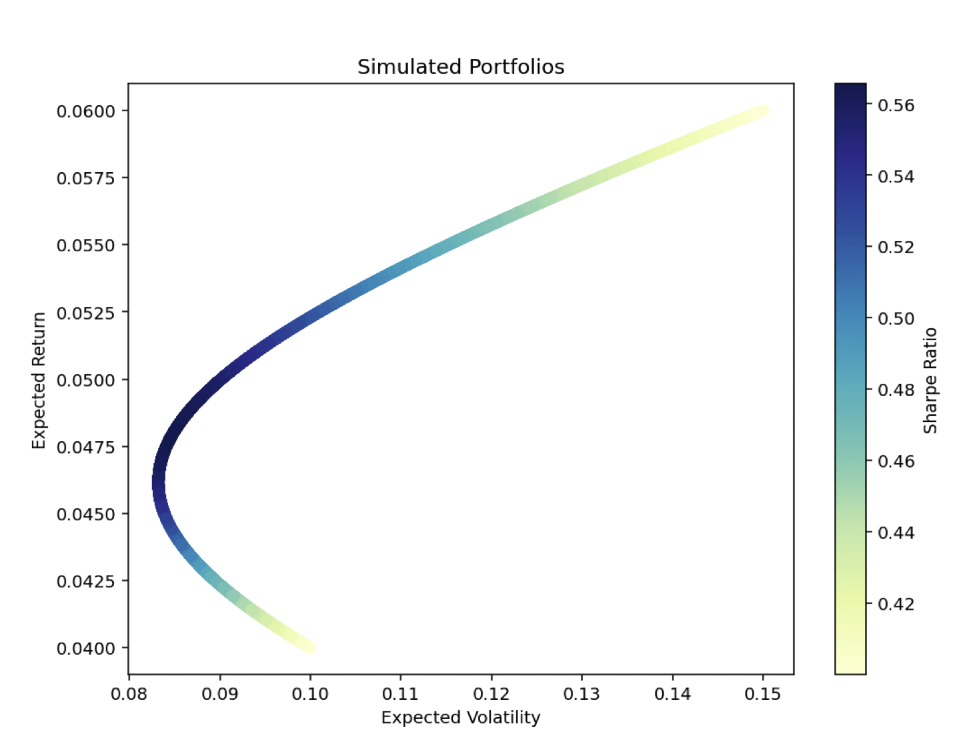
The simulation generated a wide range of possible portfolios, indicated by the plot above.

Each point represents a portfolio with a specific combination of stocks and bonds, showing its expected return and volatility.

The color indicates the Sharpe Ratio, which is the return per unit of risk.

The optimal portfolio was found using mean-variance optimization, focusing on maximizing the Sharpe ratio.

It suggests an allocation of about 40% to stocks and 60% to bonds to achieve the best risk-adjusted return given the 0% correlation between stocks and bonds and their respective returns expectations and volatility, with an expected annual return of approximately 4.80% and a volatility of 8.49% (for the entire portfolio).

This makes sense because the information we fed it was that stocks are 50% more volatile (15% vs. 10%) but with 50% higher return (6% vs. 4%).

So to balance the two we should put 60% in bonds and 40% in stocks.

This allocation balances the higher returns of stocks with the lower volatility of bonds.

This optimizes for a portfolio that has a relatively low risk for its level of expected returns.

Conclusion

Covariance and correlation are important concepts and metrics in asset allocation, used for diversification and risk management.

Understanding and effectively applying these concepts can significantly enhance trading/investment strategy and portfolio performance.

One of the most important things to understand is that correlations and covariances are not static.

They change over time due to economic shifts, policy changes, and other factors.

Regular reassessment of these measures is important for effective asset allocation.