Stochastic Processes in Financial Markets (Components, Forms)

Stochastic processes are mathematical models used to predict the probability of various outcomes over time, accounting for random variables and unknowns.

In finance, they are used in forecasting market trends and asset prices, helping traders/investors to make informed decisions and manage risks effectively.

 

---

Key Takeaways – Stochastic Processes in Financial Markets

• Understanding Uncertainty:
  • Stochastic processes are used for modeling the behavior of asset prices, interest rates, and other financial instruments.
  • They provide a mathematical framework for analyzing and predicting the probable future paths of prices.
• Risk Management:
  • Allows financial analysts to estimate the probability of different outcomes in the markets.
  • Helps in the pricing of derivative securities.
• Optimization of Trading and Investment Strategies:
  • Stochastic processes contribute to strategy optimization via the simulation of various scenarios -> assessing the potential impact on portfolios.
  • We cover various techniques below.

---

 

Components of a Stochastic Process

A stochastic process is characterized by several components:

1) State Space

The set of all possible outcomes or states that the process can assume.

Example

In stock price modeling, the state space could be the possible range of prices the stock can have.

2) Index Set

The parameter that defines the progression of time or space in the process.

Example

In a time series analysis, the index set could be discrete (days, months) or continuous (time in seconds).

3) Random Variables

Variables that can take on different values with certain probabilities, representing the randomness inherent in the process.

Example

The daily returns of a stock, where the return on each day is a random variable.

4) Realizations

Specific outcomes or sequences generated by the stochastic process.

Example

A particular path of stock prices over a year, representing one realization of the stochastic process.

5) Probability Measure

A mathematical function that assigns probabilities to different outcomes or sequences in the process.

Example

The probability distribution of stock returns, which quantifies the likelihood of different levels of returns.

Understanding these components allows analysts and researchers to build models that can simulate and analyze complex systems, such as financial markets, that have a degree of uncertainty and randomness.

 

Forms of Stochastic Processes & Applications to Finance

Here are various forms of stochastic processes along with examples of how they might apply to finance:

Random Walk

A process where each step is determined by a random variable, without any predictable pattern.

Example

In the stock market, a random walk suggests that past movements or trends cannot be used to predict future movements, implying that stock prices are essentially random and not influenced by past trends.

Geometric Brownian Motion (or Wiener Process)

A continuous-time stochastic process characterized by continuous paths and independent, normally distributed increments.

Brownian Motion forms the basis for several other stochastic processes, particularly in the Black-Scholes option pricing model.

Example

Often used in the pricing of financial derivatives, where it helps in modeling the random behavior of asset prices over time.

Poisson Process

A counting process where the number of events occurring in any interval of time is a Poisson random variable, and the time between successive events has an exponential distribution.

Example

Employed in credit risk modeling to predict the number of defaults within a portfolio of loans over a certain period, assuming a constant average rate of defaults.

Markov Chain

A Markov Chain is a stochastic process where the probability of transitioning to any particular state depends solely on the current state and time elapsed, not on the sequence of events that preceded it.

Example

Used in modeling interest rate changes where the future interest rate depends only on the current rate and not on the path taken to reach the current rate (e.g., CIR Model, BDT Model, Chen Model).

Martingale & Semimartingale

A sequence of random variables where the expected value of the next observation, given all past observations, is equal to the present observation.

A semimartingale is a more general stochastic process that includes martingales and allows for drift, meaning the expected value can change over time.

For example, a stock price could be considered a semimartingale because you expect to have positive return (drift) over time because that’s the idea behind owning it – deriving positive expected return over time.

Example

In the context of financial markets, a martingale represents a fair game, where no information or analysis can give an investor/trader an advantage. This implies that the best prediction for tomorrow’s price is today’s price.

An example of a semimartingale is the price of a financial asset in a market with transaction costs – the price process includes both a predictable trend (drift) and an unpredictable random component.

Levy Process

A process that generalizes Brownian motion and Poisson processes and is characterized by stationary, independent increments.

Example

Used in modeling stock returns and price movements.

Especially used in the presence of jumps or sudden changes, offering a more realistic representation of financial markets.

Ornstein-Uhlenbeck Process

A mean-reverting process often used to model interest rates and other financial variables.

Example

Employed in the valuation of interest rate derivatives.

Helps to model the evolution of interest rates that tend to revert to a long-term mean.

Jump Diffusion Process

A process that incorporates both continuous paths and jumps.

Often used to model asset prices that may have sudden jumps due to news or events.

Example

Used in option pricing to incorporate the possibility of sudden, significant changes in asset prices.

Hawkes Process

A self-exciting point process used to model events that are clustered in time.

Often used in high-frequency financial data analysis.

Example

Utilized in modeling high-frequency trading strategies.

It helps in understanding the clustering of trades or quotes.

Can be used to predict periods of high activity.

Fractional Brownian Motion

A generalization of Brownian motion that incorporates memory in the process.

Characterized by a Hurst parameter that measures the degree of memory.

Example

Used in modeling financial time series with long-range dependence.

It can capture more complex structures and correlations in financial data.

Queuing Theory

Involves the study of waiting lines or queues.

Uses stochastic processes to model the time of arrival of entities and the time taken to serve them.

Example

Applied in the optimization of trading algorithms.

Helps in understanding and minimizing the latency and slippage associated with executing large orders.

In other words, has applications with respect to transaction costs.

Hidden Markov Model (HMM)

A statistical Markov model where the system being modeled is a Markov process with unobserved (hidden) states.

The term “hidden” in HMM refers to the fact that the actual state sequence the system goes through is not directly observable.

It can only be inferred from the observable data.

Example

Because this is a little abstract, let’s use a more concrete example first.

Imagine you have a friend who lives in a place where it either rains or shines every day, but you can’t see the weather directly.

However, every day, your friend carries either an umbrella or sunglasses. By observing whether your friend carries an umbrella or sunglasses over several days, you can make a guess about the weather (hidden state) on those days.

The weather is the hidden state, and the accessory (umbrella or sunglasses) is the observable data.

In the context of algorithmic trading, HMM can be used to model hidden states of the market.

These hidden states might represent different market conditions, like “fear” or “greed.”

The observable data in this case could be stock prices, trading volumes, or other market indicators.

By analyzing this data with HMM, traders can infer the hidden states of the market and design trading strategies to exploit potential opportunities.

Autoregressive (AR) Processes

In these processes, the value at a given time depends linearly on the previous values.

Example

Used in time series forecasting to predict future values of financial variables based on their past values, aiding in investment strategy formulation.

Moving Average (MA) Processes

Here, the value at a given time is a linear combination of past white noise error terms.

Example

Employed in financial time series analysis to smooth out short-term fluctuations and highlight longer-term trends or cycles.

It can assist in risk management and strategy development.

 

How to Solve Stochastic Differential Equations (SDEs)

Solving Stochastic Differential Equations (SDEs) is a task in quantitative finance, particularly for modeling asset prices, interest rates, and other financial variables.

These equations incorporate random variables to represent the inherent unknowns in financial markets.

Understanding SDEs

An SDE can generally be represented in the form:

dX = a(X, t) dt + b(X,t) dW

Where:

• X is the stochastic process we’re interested in
• a(X, t) is the drift term – e.g., annual stock returns per year
• b(X,t) is the diffusion term – e.g., the movement around the mean return in the stock
• dW represents a Wiener process or Brownian motion

Analytical Solutions

Linear SDEs

Some SDEs can be solved analytically, particularly linear ones like the Ornstein-Uhlenbeck process or the Geometric Brownian Motion (GBM), which is used in the Black-Scholes model.

For instance, the GBM SDE is given by:

dSt​= μ St​ dt + σ St​ dWt​

Where:

• St​ is the asset price
• $\mu$ is the drift rate, and
• $\sigma$ is the volatility
• Wt​ is a Wiener process or Brownian motion

Transformation Techniques

Sometimes, it’s possible to transform an SDE into a simpler form that can be solved analytically.

This often involves using methods like Ito’s Lemma to manipulate the SDE into a recognizable form.

Numerical Solutions

For most practical scenarios in finance, SDEs don’t have closed-form solutions and must be solved numerically.

Euler-Maruyama Method

This is a straightforward extension of the Euler method for ordinary differential equations.

It approximates the solution at discrete time steps.

The general form for an SDE is approximated as:

 

ΔX = Xt​ + a(Xt​,t)Δt + b(Xt​,t)ΔWt

​

Where ΔWt​ is the increment of the Wiener process, which can be simulated as a normal random variable with mean 0 and variance $\Delta t$.

Milstein Method

This method provides a better approximation than the Euler-Maruyama method by including an additional term involving the derivative of the diffusion coefficient.

It’s particularly useful when the diffusion term is non-linear.

Runge-Kutta Methods (for SDEs)

These are higher-order methods providing more accuracy at the cost of computational complexity.

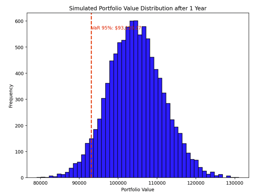
Monte Carlo Simulations

This involves simulating a large number of paths for the stochastic process and averaging the results.

It’s particularly useful for pricing complex derivatives or portfolio simulations.

It will build out a distribution like the following and can give you calculations like VaR and other risk measures:

Implementation Considerations

Choosing Time Steps

The accuracy of the numerical solution heavily depends on the choice of time steps.

Smaller time steps increase accuracy but also computational cost.

Random Number Generation

Quality of the random number generator is important, especially for Monte Carlo simulations.

Stability and Convergence

Ensure the numerical method is stable and converges to the true solution as the time step decreases.

Programming Languages

Python, with libraries like NumPy and SciPy, is commonly used for prototyping due to its ease of use. (Python packages like SymPy, and SDEPy are also commonly used for solving SDEs.)

For performance-intensive tasks, C++ or Scala may be preferred.

Summary

The choice of method for solving an SDE depends on the specific equation and the context in which it’s being used.

Analytical solutions are preferred for their precision, but numerical solutions are more versatile and widely applicable in complex real-world scenarios in finance.

 

Stochastic Process & Stochastic Calculus – Python Examples (Stock Price Estimation)

Stochastic processes and stochastic calculus are fundamental in modeling the random behavior of asset prices.

We’ll provide a couple coding examples.

As mentioned above, one of the most widely used models for stock price dynamics is the Geometric Brownian Motion (GBM), which is a continuous-time stochastic process.

The GBM is used in the Black-Scholes model, among others, for option pricing.

Here’s a simplified overview of how a stock price might be modeled using GBM:

#1 Geometric Brownian Motion (GBM)

The GBM assumes that the logarithm of the price of the stock follows a Brownian motion with drift.

It is defined by the stochastic differential equation (SDE):

 

dSt​= μ St​ dt + σ St​ dWt

​

Where:

• St​ is the asset price
• $\mu$ is the drift rate, and
• $\sigma$ is the volatility
• Wt​ is a Wiener process or Brownian motion

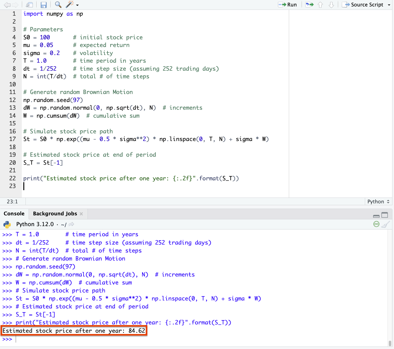
Here’s how you could estimate the price of a stock one year in the future using Python, assuming Geometric Brownian Motion:

 

import numpy as np

# Parameters
S0 = 100       # initial stock price
mu = 0.05      # expected return
sigma = 0.2    # volatility
T = 1.0        # time period in years
dt = 1/252     # time step size (assuming 252 trading days)
N = int(T/dt)  # total # of time steps

# Generate random Brownian Motion
np.random.seed(97)  
dW = np.random.normal(0, np.sqrt(dt), N)  # increments
W = np.cumsum(dW)  # cumulative sum

# Simulate stock price path
St = S0 * np.exp((mu - 0.5 * sigma**2) * np.linspace(0, T, N) + sigma * W)

# Estimated stock price at end of period
S_T = St[-1]

print("Estimated stock price after one year: {:.2f}".format(S_T))

 

In this particular simulation, we got a stock price of 84.62 at the end of one year (so slightly unlucky relative to our starting price of 100).

 

 

Important Points

• Practical Use: In reality, you’d use historical data to estimate the parameters $\mu$ and $\sigma$ for a particular stock.
• Limitations: GBM assumes constant drift and volatility, which may not hold in real-world markets. More complex models like stochastic volatility models or jump diffusion models might be used for more accurate or realistic scenarios.
• Risk & Uncertainty: It’s critical to understand the assumptions and limitations before using it for real trading/investment decisions.

Simulation (Euler-Maruyama Method)

The Euler-Maruyama method is a numerical technique used to solve stochastic differential equations (SDEs) like the Geometric Brownian Motion (GBM) equation for stock prices.

It’s essentially the stochastic equivalent of the Euler method for ordinary differential equations, adapted to handle the random component introduced by the Brownian motion.

This involves discretizing the time into small intervals and iteratively updating the price.

Here’s how you would implement the Euler-Maruyama method in Python to estimate the future stock price using GBM:

1. Discretize the time interval into small increments.
2. Iteratively update the stock price using the GBM formula at each time step.

The stochastic differential equation for GBM is:

 

dSt​= μ St​ dt + σ St​ dWt

 

To simulate this using the Euler-Maruyama method, you discretize it as follows:

 

S(t+Δt) ​= St ​+ μSt​Δt + σSt(√Δt)​Zt​

 

Here, Zt​ is a random variable from the standard normal distribution, representing the increment of the Wiener process.

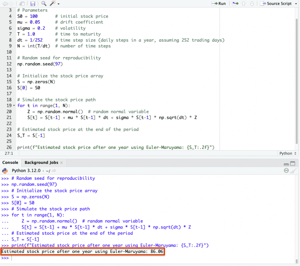
So, here’s the Python code using Euler-Maruyama for one-year future stock price estimation:

import numpy as np

# Parameters
S0 = 100 # initial stock price
mu = 0.05 # drift coefficient
sigma = 0.2 # volatility
T = 1.0 # time to maturity
dt = 1/252 # time step size (assuming 252 trading days)
N = int(T/dt) # number of time steps

# Random seed (do same as above)
np.random.seed(97)

# Initialize the stock price array
S = np.zeros(N)
S[0] = S0

# Simulate the stock price path
for t in range(1, N):
Z = np.random.normal() # random normal variable
S[t] = S[t-1] + mu * S[t-1] * dt + sigma * S[t-1] * np.sqrt(dt) * Z

# Estimated stock price at the end of the period
S_T = S[-1]

print(f"Estimated stock price after one year using Euler-Maruyama: {S_T:.2f}")

 

And we get 86.06 from this method:

 

 

Important Points

Like we did in the last section:

• Accuracy: The accuracy of the Euler-Maruyama method depends on the size of the time step $\Delta t$. Smaller time steps generally lead to more accurate simulations but require more computations.
• Parameters: In practice, you’d estimate $\mu$ (drift) and $\sigma$ (volatility) from historical data of the stock.
• Risk and Limitations: Like all models, this is a simplification of reality. Real stock prices may exhibit jumps, mean reversion, or stochastic volatility, which aren’t captured by the simple GBM model. Always be mindful of the model’s assumptions and limitations when making real-world trading decisions.

 

Below we categorize stochastic processes by type:

Discrete Time

Bernoulli Process

A sequence of independent binary random variables.

Typically represents a series of trials with only two possible outcomes.

Branching Process

A model describing a population in which each individual in one generation independently produces a random number of offspring forming the next generation.

Chinese Restaurant Process

A probability model where new individuals join a group based on the size of existing groups.

Analogous to customers choosing tables in a Chinese restaurant.

Galton–Watson Process

A process modeling population dynamics where each individual in a generation independently produces a random number of offspring for the next generation.

Independent & Identically Distributed Random Variables

A sequence of random variables that are all drawn from the same probability distribution and are mutually independent.

Markov Chain

A stochastic process where the probability of each event depends only on the state attained in the previous event.

Moran Process

A process describing the evolution of a population’s genetic composition, where individuals are replaced at random with offspring of others.

Random Walk (Variants include Loop-erased, Self-avoiding, Biased, Maximal entropy)

A stochastic process describing a path consisting of a succession of random steps, with variants introducing specific rules or biases to the walk’s properties.

Loop-erased Random Walk

A random walk where loops, paths that return to a previously visited point, are continuously removed as they form.

Results in a self-avoiding path.

Self-avoiding Random Walk

A random walk that never visits the same point more than once, effectively avoiding its own path.

Biased Random Walk

A random walk where the probability of taking a particular step is not uniform but biased in one or more directions.

Leads to a tendency to drift towards certain areas.

Maximal Entropy Random Walk

A random walk that maximizes the entropy of the visitation frequency distribution.

Often results in paths that explore the space more uniformly compared to classical random walks.

 

Continuous Time

Additive Process

A stochastic process where increments are independent and the distribution of increments is independent of the time parameter.

Bessel Process

A stochastic process representing the radial part of Brownian motion.

Describes the distance from the origin in multidimensional space.

Birth–Death Process (Pure Birth)

A stochastic process modeling populations where each individual may give birth to new individuals or die, with the “pure birth” case excluding deaths.

Brownian Motion (Bridge, Excursion, Fractional, Geometric, Meander, Cauchy process)

A fundamental continuous-time stochastic process describing random motion, with variations:

Bridge

Brownian motion conditioned to return to the origin at a fixed future time.

Excursion

A Brownian motion starting at zero, ending upon returning to zero, and remaining positive in between.

Fractional

Generalization of Brownian motion with a specified level of “memory” or correlation between increments.

Geometric

A stochastic process obtained by exponentiating Brownian motion, often used in financial modeling.

Meander

A Brownian motion that is positive over a fixed interval and conditioned not to return to the origin.

Cauchy Process

A variation of Brownian motion with increments following a Cauchy distribution.

Contact Process

A stochastic process representing the spread of an infection in a population where individuals are in “contact” with their neighbors.

Continuous-time Random Walk

A generalization of the random walk process to continuous time.

Often used to model anomalous diffusion.

Cox Process

A stochastic process generalizing the Poisson process with a time-varying rate function that is itself a random process.

Diffusion Process

A continuous-time stochastic process with continuous paths.

Often used to model particles undergoing diffusion.

Dyson Brownian Motion

A stochastic process describing the eigenvalues of a matrix as they evolve over time according to Brownian motion.

Empirical Process

A process formed by the cumulative distribution function of a sample from a population, relative to the true cumulative distribution function.

Feller Process

A strong Markov process with continuous paths, which fulfills certain technical conditions regarding its transition probabilities.

Fleming–Viot Process

More traditionally used in biology rather than finance, a Fleming-Vlot Process is a stochastic process describing the evolution of allele frequencies in a population with resampling.

Gamma Process

A process with independent increments where the time between events follows a gamma distribution.

Geometric Process

A stochastic process where each increment is geometrically distributed.

Hawkes Process

A self-exciting point process where the occurrence of an event increases the rate of future events in a cluster-like manner.

Hunt Process

A generalization of Markov processes incorporating a broader range of stochastic behaviors.

Interacting Particle Systems

Systems of particles where the behavior of each particle is dependent on the states of other particles in its neighborhood.

Itô Diffusion

A type of stochastic process with continuous paths and stochastic differential equations driven by Brownian motion.

Itô Process

A general stochastic process used in the Itô calculus.

Incorporates both drift and diffusion components.

Jump Diffusion

A stochastic process combining both continuous diffusion and discrete jumps at random times.

Used to better model financial asset prices.

Jump Process

A stochastic process with discrete changes or “jumps” occurring at random times.

Lévy Process

A process with stationary, independent increments.

Generalizes Brownian motion and Poisson processes.

Local Time

A stochastic process quantifying the amount of time a Brownian path or similar process spends at a particular location.

Markov Additive Process

A process with Markovian properties where the addition of increments depends on the current state of a background Markov process.

McKean–Vlasov Process

A stochastic process where the distribution of future states depends on the current distribution of states among all particles or individuals.

Ornstein–Uhlenbeck Process

A process describing the velocity of a particle undergoing Brownian motion.

Often used to model mean-reverting phenomena.

An example would be the mean-reversion used in the Vasicek Model.

Also used in quantitative finance for modeling certain commodity prices.

Poisson Process (Compound, Non-homogeneous)

A Poisson Process, whether compound or non-homogeneous, describes a sequence of events occurring randomly over time, with the compound version accounting for events that can have varying impacts, and the non-homogeneous version allowing the event rate to change over time.

Compound

Each event leads to multiple outcomes or “marks.”

Non-homogeneous

The rate of event occurrence varies over time.

Schramm–Loewner Evolution

A stochastic process describing the scaling limits of loop-erased random walks and related models in the complex plane.

Semimartingale

A generalization of martingales, allowing for certain “well-behaved” discontinuities in the process.

Sigma-Martingale

A Sigma-Martingale is a mathematical model used in financial mathematics to describe the evolution of an asset’s price.

Ensures that its expected value, adjusted for risk, remains constant over time, facilitating fair pricing in markets.

Stable Process

A process characterized by stable distributions, which are a generalization of the normal distribution.

Superprocess

A measure-valued stochastic process generalizing branching processes and interacting particle systems.

Telegraph Process

A process that alternates between two different states or velocities.

Resembles the signals in a telegraph wire.

Variance Gamma Process

A process with increments following the variance-gamma distribution

Often used to model financial returns.

Wiener Process

Another name for Brownian motion, a continuous-time stochastic process with independent, normally distributed increments.

Wiener Sausage

The volume traced out by a sphere (or circle in 2D) moving according to Brownian motion over a fixed time interval.

 

Both Discrete Time & Continuous time

Branching Process

A process modeling population dynamics, where each individual in one generation independently produces a random number of offspring

Applicable in both discrete (e.g., Galton-Watson process) and continuous time (e.g., age-dependent branching processes).

Galves–Löcherbach Model

A model for interacting neuron dynamics where the potential of each neuron evolves according to a stochastic process influenced by the spiking of other neurons.

Gaussian Process

A collection of random variables, any finite number of which have a joint Gaussian distribution, used in various fields such as machine learning and spatial statistics.

Hidden Markov Model (HMM)

A statistical model where the system being modeled is assumed to follow a Markov process with unobservable (hidden) states

Used in various temporal pattern recognition scenarios, applicable in discrete time but with extensions to continuous time.

Markov Process

A stochastic process that satisfies the Markov property (future states depend only on the current state, not on the sequence of events that preceded it).

Applicable in both discrete and continuous time as Markov chains or Markov processes, respectively.

Martingale (Differences, Local, Sub-, Super-)

A model for a fair game, where the conditional expected value of the next observation, given all past observations, is equal to the most recent observation, with various forms:

Differences Martingale

A process where the difference between successive terms is a martingale.

Local Martingale

A process that resembles a martingale in a local sense but may not be a true martingale globally.

Sub-Martingale

A process where the conditional expected future value, given the present and past, is at least as large as the present value.

Super-Martingale

A process where the conditional expected future value, given the present and past, is at most equal to the present value.

Random Dynamical System

A dynamical system in which the evolution rule incorporates randomness.

Regenerative Process

A process that has certain points in time (regeneration points) at which the probabilistic behavior of the future is independent of the past.

Renewal Process

A counting process that models the times at which events occur, with the times between events being independent and identically distributed.

Stochastic Chains with Memory of Variable Length

A generalization of Markov chains where the probability of transitioning to the next state may depend on a variable-length history of past states.

Applicable in discrete time with potential continuous time adaptations.

White Noise

A random signal having equal intensity at different frequencies, used as a basic input in many systems.

Used in both discrete (sequences of uncorrelated random variables) and continuous time (as a model for stochastic processes like Brownian motion).

 

Fields of Stochastic Processes

Dirichlet Process

A probability distribution over probability distributions, used in Bayesian nonparametric statistics to allow for unknown numbers of underlying components in a mixture model.

Gaussian Random Field

A generalization of Gaussian processes to multi-dimensional spaces, where each point in the space is associated with a random variable, and the collection of these variables has a multivariate normal distribution.

Gibbs Measure

A probability measure used in statistical mechanics and the study of Markov random fields.

Characterizes the distribution of states of a system based on the energy of each configuration and a temperature parameter.

Hopfield Model

A type of recurrent artificial neural network that serves as a content-addressable memory system with binary threshold nodes.

Models the way neurons in the brain function to store and retrieve memories.

Ising Model (Potts model, Boolean network)

A mathematical model of ferromagnetism in statistical mechanics, with extensions:

Potts Model

A generalization of the Ising model allowing more than two possible states per site.

Boolean Network

A network of nodes with binary states, with each node’s state determined by a fixed Boolean function of the states of some set of nodes.

Markov Random Field

A set of random variables having a Markov property described by an undirected graph.

Used in spatial statistics, image processing, and machine learning to model complex interactions between variables.

Percolation

A mathematical theory studying the movement and filtering of fluids through porous materials, used to model the behavior of connected clusters in a random graph.

Pitman–Yor Process

A stochastic process generalizing the Dirichlet process, providing a framework for Bayesian nonparametric models, particularly allowing for power-law behavior in the number of clusters as more data is observed.

Point Process (Cox, Poisson)

A type of random process for the description and modeling of random points in time or space, with specific types:

Cox Process (Doubly Stochastic Poisson Process)

A generalization of the Poisson process where the intensity itself is a random function.

Poisson Process

A simple and widely used type of point process that models random events occurring independently and uniformly over time or space.

Random Field

A generalization of a stochastic process to multiple dimensions, where each point in a space is associated with a random variable.

Random Graph

A graph that is generated by some random process.

Used in various fields to study network structures in physical, biological, and information systems, including the internet and social networks.

 

Time Series Models Using Stochastic Processes

Autoregressive Conditional Heteroskedasticity (ARCH) Model

A time series model used to characterize and model observed time series data with time-varying volatility.

Captures periods of swings followed by periods of relative calm.

Autoregressive Integrated Moving Average (ARIMA) Model

A generalization of the simpler Autoregressive Moving Average (ARMA) model that can be applied to time series data that are non-stationary, made stationary by differencing the data one or more times.

Autoregressive (AR) Model

A time series model where future values are assumed to be a linear combination of past values and a stochastic term.

Emphasizes that past values have an effect on future values.

Autoregressive–Moving-Average (ARMA) Model

A time series model blending the Autoregressive (AR) and Moving-Average (MA) models.

Captures both the momentum and mean reversion effects in time series data.

Generalized Autoregressive Conditional Heteroskedasticity (GARCH) Model

An extension of the ARCH model that provides a more flexible approach to modeling time series data with time-varying volatility.

Accounts for not just the lagged conditional variances but also the lagged squared observations.

Moving-average (MA) Model

A time series model where future values are assumed to be a linear combination of past error terms (shocks or white noise).

Models the idea that random shocks can influence future values of a series.

 

Financial Models Using Stochastic Processes

Binomial Options Pricing Model

A discrete-time model for valuing options that divides time into a series of intervals and computes the option value at each point using a lattice-based approach.

Black–Derman–Toy Model

A one-factor interest rate model that describes the evolution of interest rates by modeling their future expected values and volatility.

Black–Karasinski Model

A log-normal interest rate model that preserves the analytical tractability of interest rate caps, floors, and swaptions.

Black–Scholes Model

A mathematical model for the dynamics of a financial market containing derivative investment instruments.

Primarily used for pricing European options.

Related: Modeling Black-Scholes in R and MATLAB

Chan–Karolyi–Longstaff–Sanders (CKLS) Model

A generalized model of interest rate dynamics that allows the volatility of the short rate to be a function of the level of the short rate itself.

Chen Model

A model of interest rate dynamics that incorporates stochastic volatility and the mean reversion feature of interest rates.

Constant Elasticity of Variance (CEV) Model

A financial model that describes the evolution of a security’s volatility as a function of its price levels.

Cox–Ingersoll–Ross (CIR) Model

A mathematical formula used to model the evolution of interest rates that is an extension of the Vasicek model.

Incorporates a square root to ensure that interest rates do not become negative.

Garman–Kohlhagen Model

An adaptation of the Black–Scholes model for pricing foreign exchange options.

Heath–Jarrow–Morton (HJM) Framework

A framework for modeling forward rates that directly specifies the dynamics of forward rates under a risk-neutral measure.

Heston Model

A mathematical model describing the evolution of volatility in the financial market, where volatility itself is treated as a stochastic process.

Ho–Lee Model

The first arbitrage-free model for interest rate derivatives, which models the evolution of interest rates.

Hull–White Model

An extension of the Vasicek and CIR models of interest rate dynamics.

Adds in time-dependent parameters for the mean reversion and volatility rate.

LIBOR Market Model

A financial model of interest rates which incorporates multiple factors.

Models the evolution of the forward LIBOR rates (or LIBOR-like rates since LIBOR is now defunct) rather than instantaneous interest rates.

Rendleman–Bartter Model

A model for pricing bonds and bond options.

Assumes that interest rates are stochastic with a certain drift and volatility.

SABR Volatility Model

A stochastic volatility model that captures the volatility smile in derivatives markets, where both the price and volatility are treated as stochastic processes.

Vasicek Model

An early model describing the evolution of interest rates, which assumes that the movement of interest rates is subject to random fluctuations and mean reversion.

Wilkie Model

A stochastic asset model for actuarial use.

Focuses on the long-term investment returns of equities, bonds, cash, and inflation.

 

Actuarial models

Bühlmann Model

A mathematical framework used in actuarial science for experience rating, which combines the overall population experience with individual experience to price insurance premiums more accurately.

Cramér–Lundberg Model

A classic model in actuarial risk theory, often referred to as the “Poisson risk model.”

Used to describe the process of incoming insurance claims and the capital of an insurance company over time.

Risk Process

A stochastic model representing the capital of an insurance company.

Accounts for premium income and claim payments over time.

It’s fundamental in the quantification and management of risk in insurance and finance.

Sparre–Anderson Model

A generalization of the Cramer–Lundberg model in actuarial science.

Allows for arbitrary inter-arrival times of claims which are independent and identically distributed, but not necessarily exponentially distributed (which is a key assumption in the Cramer–Lundberg model).

 

Queueing Models

Queueing models in finance are used to analyze and optimize the flow of transactions, such as order executions and clearing processes, to improve efficiency and manage congestion in financial markets.

Bulk Queue

A queueing model where customers arrive and are serviced in batches or “bulks” rather than individually.

Often applied in situations like batch processing or bulk buying.

Fluid Queue

A queueing model that treats the content (e.g., customers, data packets) as a continuous “fluid.”

Allows for the analysis of systems where discrete packet arrivals and services can be approximated by continuous flows.

Generalized Queueing Network

A network of interconnected queues where the output from one queue can become the input to another.

Used to model complex systems with multiple stages of service or interaction.

M/G/1 Queue

A single-server queueing model where arrivals follow a Poisson process (“M” denotes Markovian or memoryless inter-arrival times), service times are generally distributed (“G” denotes General distribution), and there is one server.

M/M/1 Queue

A basic queueing model with a single server where both arrival and service times follow exponential distributions (“M” denotes Markovian or memoryless), leading to a simple and analytically tractable model.

M/M/c Queue

A generalization of the M/M/1 queueing model with multiple servers (“c” denotes the number of servers), where arrivals follow a Poisson process, and service times are exponentially distributed.

This model is useful for analyzing systems with parallel servers or channels.

 

Properties

Càdlàg Paths

Functions defined on the real line that are right-continuous and have left limits.

Often used in the study of stochastic processes (the term is an acronym from the French “continu à droite, limites à gauche”).

Continuous

A property of a function or process where small changes in the input lead to small changes in the output, without sudden jumps or discontinuities.

Continuous Paths

In the context of stochastic processes, this refers to processes where sample paths are continuous functions of time, such as in standard Brownian motion.

Ergodic

A property of a stochastic process where time averages converge to ensemble averages.

Implies that the process’s long-term behavior is independent of its initial state.

Exchangeable

A property of a sequence of random variables where the joint probability distribution is invariant under permutations.

In other words, the order of the variables doesn’t affect the distribution.

Feller-Continuous

A property of a Markov process where the transition probabilities are continuous with respect to the initial state.

Ensures that the process’s behavior changes smoothly as the initial state changes.

Gauss–Markov

A stochastic process or a sequence of random variables that has the least-variance property among all linear unbiased estimators.

Often used in the context of the linear regression model.

Markov

A property of a stochastic process where the future state depends only on the current state and not on the sequence of events that preceded it, known as the “memoryless” property.

Mixing

A property of a stochastic process indicating a strong form of stochastic independence over time.

Implies that the past and future events become increasingly independent as the time interval between them grows.

Piecewise-Deterministic

A type of stochastic process that is deterministic between random events, at which times the process may change direction abruptly or jump.

Predictable

A property of a stochastic process where future values can be predicted with no error based on current and past values and information.

Progressively Measurable

A property of a stochastic process where, up to any fixed time, the process’s past behavior is measurable with respect to the information available up to that time.

Self-Similar

A property of a process where the statistical properties are invariant under scaling of time or space.

Typically used in the context of fractals or certain types of stochastic processes like fractional Brownian motion.

Stationary

A property of a stochastic process where the joint probability distribution doesn’t change when shifted in time.

Implies that statistical properties like the mean and variance are constant over time.

Time-Reversible

A property of a stochastic process where the process behaves the same way forward in time as it does in reverse – i.e., the statistical behavior is the same when time is reversed.

 

Limit Theorems

Central Limit Theorem

States that the distribution of the sum (or average) of a large number of independent, identically distributed random variables approaches a normal distribution, regardless of the original distribution of the variables.

Donsker’s Theorem

Often referred to as the invariance principle, states that the scaled cumulative sum of a sequence of independent and identically distributed random variables converges in distribution to a Brownian motion.

Doob’s Martingale Convergence Theorems

A collection of fundamental results in the theory of martingales.

They state conditions under which martingales converge, either almost surely or in the L^p sense.

Ergodic Theorem

Describes the long-term average behavior of a dynamical system, stating that, under certain conditions, the time average of a function along the trajectories of the system equals the space average.

Fisher–Tippett–Gnedenko Theorem

Also known as the Extreme Value Theorem, it characterizes the asymptotic behavior of extreme values (maxima or minima) of a sample of independent and identically distributed random variables.

Large Deviation Principle

Provides a framework for estimating probabilities of rare events in a wide range of stochastic processes.

Quantifies the rate at which probabilities decay to zero.

Law of Large Numbers (weak/strong)

Describes the result of performing the same experiment a large number of times.

States that the sample average converges to the expected value:

Weak Law

Convergence in probability.

Strong Law

Almost sure convergence.

Law of the Iterated Logarithm

Describes the precise asymptotic behavior of the maximal deviation of a random walk.

States that the fluctuations of a random walk are almost surely bounded by a function involving the iterated logarithm.

Maximal Ergodic Theorem

Provides conditions under which the time average of a function along the trajectories of a dynamical system is almost surely non-negative, given that its space average is non-negative.

Sanov’s Theorem

A result in the theory of large deviations concerning the probability of observing an atypical empirical distribution of independent and identically distributed random variables.

Zero–One Laws (Blumenthal, Borel–Cantelli, Engelbert–Schmidt, Hewitt–Savage, Kolmogorov, Lévy)

A collection of results stating that certain events in a probability space have a probability of either zero or one:

Blumenthal’s 0-1 Law

Concerns the probability of certain events related to Brownian motion at the origin.

Borel–Cantelli Lemma

Describes the conditions under which the probability of infinitely many events occurring is zero or one.

Engelbert–Schmidt Zero-One Law

Specific to stochastic processes and their behavior.

Hewitt–Savage 0-1 Law

A generalization of Kolmogorov’s 0-1 law.

Applicable in the context of exchangeable random variables.

Kolmogorov’s 0-1 Law

States that certain tail events either happen almost surely or almost never.

Lévy’s Zero-One Law

Concerns the convergence of conditional probabilities to the unconditional probability as information increases.

 

Inequalities

Burkholder–Davis–Gundy Inequalities

A set of inequalities providing bounds for the moments of the maximal function of a martingale in terms of the moments of its quadratic variation.

Used in martingale theory and stochastic integration.

Doob’s Martingale Inequalities

A collection of fundamental inequalities in the theory of martingales.

Provides bounds on the probabilities of certain events related to martingales, such as the maximum value of a martingale or the tail of its last value.

Doob’s Upcrossing Inequality

An inequality providing an upper bound on the expected number of upcrossings of an interval by a submartingale.

Important in the proof of the martingale convergence theorems.

Kunita–Watanabe Inequality

A result in stochastic calculus that provides an upper bound for the covariance of two square-integrable martingales (fundamental in the theory of stochastic integration).

Marcinkiewicz–Zygmund Inequalities

A set of inequalities related to sums of independent random variables.

Provides bounds for the moments of the sum in terms of the individual moments of the summands.

Useful in the study of the convergence of random series and integrals.

 

Tools

Cameron–Martin Formula

Provides a change of measure formula in the context of Wiener space.

Fundamental to the Girsanov theorem and important in the study of transformations of Wiener processes.

Convergence of Random Variables

Refers to various modes in which sequences of random variables can converge to a random variable (e.g., almost surely, in probability, in L^p, in distribution).

Doob’s Martingale Inequalities

A collection of inequalities providing bounds on the probabilities of certain events related to martingales, such as the maximal function of a martingale.

Doleans–Dade Exponential

A process that solves a specific stochastic differential equation.

Often used in the context of the Girsanov theorem for change of measure in stochastic processes.

Doob Decomposition Theorem

States that any integrable adapted process can be uniquely decomposed into a martingale and a predictable, increasing process.

Doob–Meyer Decomposition Theorem

Extends the Doob decomposition by showing that any submartingale can be decomposed uniquely into a martingale and a predictable, increasing process.

Doob’s Optional Stopping Theorem

Provides conditions under which the expected value of a martingale at a stopping time equals its initial expected value.

Dynkin’s Formula

Provides a relationship between Markov processes and their infinitesimal generators.

Used in solving problems related to expected function values of stochastic processes.

Feynman–Kac Formula

Provides a link between partial differential equations and stochastic processes, particularly in the context of pricing options in financial mathematics.

Filtration

A family of σ-algebras representing the information available up to each point in time.

Girsanov Theorem

Describes how the dynamics of stochastic processes change when the original probability measure is changed to an equivalent probability measure.

Infinitesimal Generator

An operator that describes the limiting behavior of a Markov process as time approaches zero.

Used to solve various problems in stochastic processes.

Itô Integral

An integral for stochastic processes.

Defines integration with respect to Brownian motion or more general martingales.

Itô’s Lemma

A fundamental formula in stochastic calculus that provides a differential rule for stochastic processes.

Analogous to the chain rule in deterministic calculus.

Karhunen–Loève Theorem

A result concerning the representation of a stochastic process as an infinite series of orthogonal functions.

Fundamental in the theory of continuous-time stochastic processes.

Kolmogorov Continuity Theorem

Provides conditions under which a stochastic process has continuous paths.

Ensures the existence of a modification of the process with continuous sample paths.

Kolmogorov Extension Theorem

Provides conditions for the existence of a stochastic process with a specified set of finite-dimensional distributions.

Fundamental in the construction of stochastic processes.

Lévy–Prokhorov Metric

A metric on the space of probability measures on a given metric space.

Provides a way to quantify the “distance” between probability measures.

Malliavin Calculus

Malliavin calculus is a mathematical technique that extends the calculus of variations to stochastic processes.

Primarily used in finance for pricing derivatives by allowing the sensitivity analysis of financial models with respect to random inputs.

Martingale Representation Theorem

States that every martingale can be represented as an Itô integral with respect to a Brownian motion under certain conditions.

Optional Stopping Theorem

See Doob’s Optional Stopping Theorem.

Prokhorov’s Theorem

Provides conditions under which a family of probability measures is relatively compact.

Fundamental in the study of weak convergence.

Quadratic Variation

A process that measures the accumulated squared increments of a stochastic process. Important in the analysis of stochastic calculus.

Reflection Principle

A principle related to Brownian motion.

States that the process reflected at its first hitting time of a level has the same distribution as the original process.

Skorokhod Integral

A generalization of the Itô integral, defined for a broader class of integrands, particularly in the context of Malliavin calculus.

Skorokhod’s Representation Theorem

Provides conditions under which a sequence of random variables with distributions converging weakly can be realized on a common probability space in such a way that they converge almost surely.

Skorokhod Space

A space of càdlàg functions equipped with the Skorokhod topology.

Used in the study of processes with jumps.

Snell Envelope

The smallest supermartingale dominating a given process.

Most often used in optimal stopping problems.

Stochastic Differential Equation (Tanaka)

Refers to differential equations involving stochastic processes, with Tanaka’s formula providing a solution for stochastic differential equations driven by semimartingales.

Here is the Tanaka stochastic differential equation:

• dξt = σ(ξt)dWt + dLt

Where:

• ξt – The stochastic process
• σ(ξt) – The state-dependent volatility function
• dWt – The increment of a standard Wiener process
• dLt – The local time or instantaneous reflection measure at the origin to keep the process ξt nonnegative.

The key aspect is the local time term dLt which pushes the stochastic process ξt back upward if it hits the origin boundary. This ensures it stays nonnegative.

This allows stochastically modeling nonnegative quantities like prices or volatilities.

Stopping Time

A random variable representing the time at which a given stochastic process first exhibits a certain behavior.

Stratonovich Integral

An alternative to the Itô integral, where the integrand is evaluated at the midpoint of the intervals. Leads to different integration properties.

Uniform Integrability

A property of a family of random variables ensuring that their expected values converge.

Fundamental in the convergence of martingales.

Usual Hypotheses

Conditions commonly imposed in the study of stochastic processes.

Ensures the existence of certain properties like càdlàg modifications and completeness of filtrations.

Wiener Space (Classical · Abstract)

Refers to the space of real-valued continuous functions on a specific interval, equipped with the Wiener measure, with:

Classical Wiener Space

The space of continuous functions on a closed interval starting at zero.

Abstract Wiener Space

A generalization of the classical Wiener space to infinite-dimensional spaces.

 

Disciplines

Actuarial mathematics

The study of mathematical and statistical methods to assess risk in insurance, finance, and other industries and professions.

Control theory

This is a branch of engineering and mathematics that deals with the behavior of dynamical systems with inputs, and how their behavior is modified by feedback.

Econometrics

Econometrics combines economics, mathematics, and statistics to analyze economic data and test hypotheses related to economic relationships.

Ergodic theory

Ergodic theory is a branch of mathematics that studies statistical properties of deterministic dynamical systems through long-term average behavior of systems over time.

Extreme value theory (EVT)

EVT focuses on the statistical analysis of the most extreme deviations from the median or mean of probability distributions.

Often applied to assess risk for rare events.

Large deviations theory

This theory provides a framework for assessing the probabilities of rare events occurring in stochastic systems (systems subject to random forces).

Machine learning

Machine learning is a field of artificial intelligence that uses algorithms and statistical models to enable computer systems to improve their performance on a specific task through experience.

Mathematical finance

Mathematical finance applies mathematical methods to financial markets and securities, often for the purpose of pricing financial derivatives.

Mathematical statistics

Mathematical statistics involves the application of mathematics to statistics, which includes the theoretical underpinnings of statistical inference and analysis.

Probability theory

Probability theory is the branch of mathematics that deals with the analysis of random phenomena and the likelihood of different outcomes.

Queueing theory

Queueing theory examines the behavior of waiting lines or queues to make predictions about queue lengths and waiting times.

Renewal theory

Renewal theory is a branch of probability theory that analyzes the times at which a system restarts or renews.

Provides a framework for understanding random processes.

Ruin theory

In actuarial science, ruin theory studies the risk that an entity’s financial reserves are depleted by claims or other financial demands, leading to insolvency.

Signal processing

Signal processing is the engineering discipline that focuses on the analysis, modification, and synthesis of signals such as sound, images, and biological measurements.

Stochastic analysis

Stochastic analysis is a branch of mathematical analysis that deals with processes involving randomness and uses methods of calculus and differential equations.

Time series analysis

Time series analysis involves statistical techniques for analyzing time-ordered data to extract meaningful statistics and characteristics of the data.

 

FAQs – Stochastic Process in Markets

How does Ito’s Lemma help in pricing stocks and other securities?

Ito’s Lemma is a concept in stochastic calculus that helps in pricing derivatives.

It provides a way to understand how the prices of financial derivatives change in response to small changes in the price of the underlying asset.

It allows for the calculation of the expected price of derivatives in a world where prices are constantly fluctuating.

What is the role of stochastic differential equations in predicting stock prices and managing financial risks?

Stochastic differential equations (SDEs) are used to model the behavior of stock prices and other financial variables that are influenced by both deterministic trends and random fluctuations.

By solving these equations, analysts can make predictions about future price movements and assess the associated risks.

How do models that consider changing volatility improve options pricing?

Models that account for changing volatility, or stochastic volatility models, offer a more realistic approach to options pricing by acknowledging that volatility itself can be unpredictable.

This leads to more accurate pricing of options.

It considers the potential future changes in volatility, helping traders avoid mispricing and make better hedging decisions.

How do models that consider multiple factors provide a better view of market trends and stock price movements?

Multi-factor models consider various sources of risk and return in the financial markets.

Accounting for multiple factors provides a more comprehensive and accurate view of market dynamics.

What is Girsanov’s Theorem and how does it relate to pricing in the financial markets?

Girsanov’s Theorem is a mathematical concept used in the change of measure techniques, which are used for pricing financial derivatives.

It allows for the conversion of probabilities from the real-world measure to the risk-neutral measure – under which the expected return on the asset is the risk-free rate.

What is the Martingale Representation Theorem and how does it help in making hedging decisions?

The Martingale Representation Theorem provides a way to represent contingent claims as stochastic integrals.

It helps in determining the portfolio processes that can hedge against the risks associated with holding certain financial positions.

Ultimately the goal is more effective and efficient risk management strategies.

What are jump-diffusion models and how do they help in understanding stock market movements?

Jump-diffusion models are used in finance to account for sudden, unexpected changes in asset prices – in addition to the usual random fluctuations.

These models help in understanding and quantifying the impact of significant market events on asset prices.

They provide a more complete picture of market dynamics rather than relying mostly on continuous models.

As such, they can help in the development of strategies to navigate such events.

How do stochastic processes help in creating and analyzing trading algorithms?

Stochastic processes are used in the development and analysis of algorithmic trading strategies by modeling the movements of asset prices.

They help in simulating various market scenarios to test and optimize trading algorithms, ensuring that the strategies are robust if deployed in the real world.

What is stochastic dominance and how does it help in making investment decisions?

Stochastic dominance is a concept used to compare the performance of different investment opportunities.

It helps traders/investors make more informed decisions by providing a framework to evaluate and rank different investment options based on their probability distributions.

This allows them to choose investments that offer better prospects of returns and risk management.

What is the Feynman-Kac theorem and how is it used in pricing financial derivatives?

The Feynman-Kac theorem connects partial differential equations and stochastic processes.

It provides a method to solve certain types of partial differential equations using expectations of stochastic processes.

This theorem is used in finance to find the prices of financial derivatives by solving the associated partial differential equations.

It offers a tool for pricing a wide range of financial instruments.

How does the Feynman-Kac formula helps in solving SDEs?

The Feynman-Kac formula provides a link between stochastic differential equations (SDEs) and partial differential equations (PDEs).

It allows one to solve certain SDEs by instead solving a corresponding PDE, specifically transforming the problem of finding the expected value of a stochastic process into a PDE problem.

This approach is particularly useful in finance for pricing derivative securities, where the PDE derived from the Feynman-Kac formula often corresponds to the Black-Scholes equation or similar models.

 

Conclusion

These processes serve as foundational tools in the analysis and modeling of financial time series and various phenomena in financial markets.

They help in risk management, option pricing, trading/investment strategy formulation, and more.