How to Model the Term Structure of Interest Rates & Credit Spreads

Modeling the term structure of interest rates and credit spreads is a fundamental task for risk managers and those who trade rate and fixed-income securities.

Various models and methods have been developed to accurately capture and predict the behavior of interest rates and credit spreads over time.

They help understand and predict various financial phenomena, like bond pricing, risk management, and trading/investment decisions.

Key Takeaways – How to Model the Term Structure of Interest Rates & Credit Spreads

• Modeling Interest Rates – Several models attempt to capture the relationship between yield and maturity:
  • Yield Curve Models
  • Factor Models
  • No-Arbitrage Models
• Modeling Credit Spreads – Credit spreads reflect the additional yield demanded by investors for holding riskier bonds compared to risk-free rates. Here are some common approaches:
  • Reduced-Form Models
  • Structural Models
  • Term Structure of Credit Spreads
• Important Considerations
  • Joint Modeling – Many advanced models integrate both interest rate and credit spread dynamics (recognizing their interdependencies).
  • Calibration and Validation – Choosing the right model and calibrating its parameters to market data is important. Backtesting and stress testing are needed for model validation.
  • Model Complexity – The level of complexity should be balanced with the problem at hand and available data. Simpler models might be sufficient for certain tasks, while complex models might be needed for detailed analysis or risk management.
• Coding Example
  • We provide a coding example of an interest rate simulation.

1. Bootstrapping

Bootstrapping is a method used to construct a zero-coupon yield curve.

The process involves deriving the spot rates for certain maturities based on the prices of coupon-bearing instruments (usually government bonds) without any arbitrage opportunities.

Here’s a high-level overview of the bootstrapping process:

Start with Short-term Instruments

Begin with instruments that have the shortest maturity (usually Treasury bills) to get the initial spot rates.

Iterative Process

Use the spot rates derived for short-term instruments to find the spot rates for longer-term instruments.

Coupon Bonds

For bonds with coupons, discount each cash flow using the spot rates corresponding to its maturity.

The sum of these discounted cash flows should equal the bond’s market price.

Extraction of Spot Rate for Long-term Instruments

Solve for the spot rate that equates the present value of cash flows to the bond’s price.

This process is repeated iteratively to build out the yield curve for all maturities.

2. Multi-Curves

The multi-curve framework is a more recent development, most relevant in the post-2008 financial world where the assumption that different maturities have a single yield curve became inadequate.

In this approach, separate curves are constructed for:

Forward Curve

For forecasting future rates.

Discount Curve

For discounting cash flows.

This approach accounts for market distortions like the ones observed during the financial crisis, where the credit risk and liquidity premiums can vary significantly across different maturities and instruments.

3. Short-Rate Models

Short-rate models focus on modeling the instantaneous interest rate (the rate for a very short period) and derive the entire yield curve from it.

Some of the well-known short-rate models include:

Vasicek Model

Assumes that the short rate follows a mean-reverting stochastic process.

It basically attempts to model the fact that interest rates don’t stay too high or too low for long durations of time.

Cox-Ingersoll-Ross (CIR) Model

Similar to the Vasicek model but ensures that the rates are always positive (which doesn’t have to be true in real-life, no matter if nominal or real).

Hull-White Model

An extension of the Vasicek model that allows for a time-dependent mean reversion level and volatility.

These models are useful for pricing interest rate derivatives like bond options or interest rate swaps.

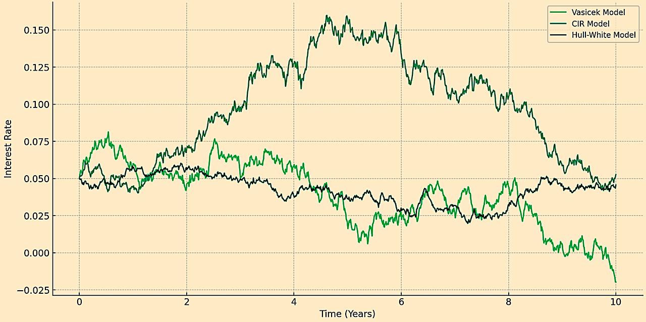
Coding Example of the Vasicek, CIR, and Hull-White Models (Short-Rate Models)

The Python code below simulates and plots the interest rates over time for three different models:

• Vasicek Model
• Cox-Ingersoll-Ross (CIR) Model, and
• Hull-White Model

Each model provides a unique approach to modeling interest rates, which reflects their respective characteristics:

• mean-reversion in the Vasicek model
• positive rates ensured by the CIR model, and
• time-dependent parameters in the Hull-White model.

import numpy as np
import matplotlib.pyplot as plt

# Parameters - Vasicek Model
r0_vasicek = 0.05 # Initial short rate
kappa_vasicek = 0.1 # Speed of mean reversion
theta_vasicek = 0.05 # Long-term mean rate
sigma_vasicek = 0.02 # Volatility
T = 10 # Time horizon
dt = 0.01 # Time step
steps = int(T / dt)
t = np.linspace(0, T, steps)

# Vasicek Model Sim
def simulate_vasicek(r0, kappa, theta, sigma, T, dt):
    steps = int(T / dt)
    rates = np.zeros(steps)
    rates[0] = r0
    for i in range(1, steps):
        dr = kappa * (theta - rates[i-1]) * dt + sigma * np.sqrt(dt) * np.random.normal()
        rates[i] = rates[i-1] + dr
    return rates

# Parameters - CIR Model
r0_cir = 0.05
kappa_cir = 0.2
theta_cir = 0.07
sigma_cir = 0.07

# CIR Model Sim
def simulate_cir(r0, kappa, theta, sigma, T, dt):
    steps = int(T / dt)
    rates = np.zeros(steps)
    rates[0] = r0
    for i in range(1, steps):
        dr = kappa * (theta - rates[i-1]) * dt + sigma * np.sqrt(rates[i-1]) * np.sqrt(dt) * np.random.normal()
        rates[i] = max(rates[i-1] + dr, 0) # Ensure rates are non-negative
    return rates

# Parameters - Hull-White Model
r0_hw = 0.05
kappa_hw = 0.08
theta_hw = lambda t: 0.05 + 0.01 * np.cos(t) # Time-dependent mean reversion level
sigma_hw = 0.01

# Hull-White Model Sim
def simulate_hull_white(r0, kappa, theta, sigma, T, dt):
    steps = int(T / dt)
    rates = np.zeros(steps)
    rates[0] = r0
    for i in range(1, steps):
        dr = kappa * (theta(t[i-1]) - rates[i-1]) * dt + sigma * np.sqrt(dt) * np.random.normal()
        rates[i] = rates[i-1] + dr
    return rates

# Simulating & plotting the models
vasicek_rates = simulate_vasicek(r0_vasicek, kappa_vasicek, theta_vasicek, sigma_vasicek, T, dt)
cir_rates = simulate_cir(r0_cir, kappa_cir, theta_cir, sigma_cir, T, dt)
hw_rates = simulate_hull_white(r0_hw, kappa_hw, theta_hw, sigma_hw, T, dt)

plt.figure(figsize=(14, 7))

plt.plot(t, vasicek_rates, label="Vasicek Model")
plt.plot(t, cir_rates, label="CIR Model")
plt.plot(t, hw_rates, label="Hull-White Model")

plt.xlabel("Time (Years)")
plt.ylabel("Interest Rate")
plt.title("Interest Rate Models Simulation")
plt.legend()
plt.show()

The plot illustrates how each model generates a path for interest rates over a 10-year horizon.

Vasicek vs. CIR vs. Hull-White Interest Rate Simulation

4. Heath-Jarrow-Morton (HJM) Framework

The HJM framework is a general framework for modeling the evolution of interest rates.

It directly models the entire forward rate curve rather than just the short rate.

Key points include:

Forward Rates

The model specifies the drift and volatility of the forward rates.

No Arbitrage

Ensures that the model is arbitrage-free.

Flexibility

Can accommodate a wide range of volatility and correlation structures.

The HJM framework is mathematically complex and computationally intensive but is highly flexible and has been used in real-world contexts.

5. Libor Market Model (LMM)

Also known as the Brace-Gatarek-Musiela model, the LMM extends the short-rate models to model the entire forward rate curve, similar to the HJM model.

It specifically models the dynamics of the various Libor rates (Libor is now defunct, so would apply to other rates) and is widely used for pricing interest rate derivatives, especially those involving Libor-like rates, like swaptions and caps/floors.

6. Cheyette Model

This is an extension of the short-rate model (particularly the Hull-White model) and it includes a stochastic volatility component.

The Cheyette model is known for its ability to capture the volatility smile effect seen in interest rate options.

7. Nelson-Siegel and Svensson Models

These are empirical models used to fit the yield curve.

The Nelson-Siegel model uses a parametric equation to describe the yield curve.

It captures the level, slope, and curvature of the curve.

The Svensson model extends this by adding another term, which allows for a better fit of the long end of the curve.

8. Cox-Ingersoll-Ross (CIR) Model Extended

This is an extension of the basic CIR model that can include multiple factors.

Allows it to capture various risk factors driving the interest rate dynamics.

9. Stochastic Volatility & Jump-Diffusion Models

These models add further complexity by incorporating features like stochastic volatility (changes in volatility over time are random) and jump diffusion (sudden, large changes in interest rates).

Examples include the Bates model and the Duffie-Darling model.

10. Arbitrage-Free Nelson-Siegel Model

This model adapts the traditional Nelson-Siegel model to ensure it’s arbitrage-free, which makes it suitable for a wider range of financial applications.

11. Dynamic Nelson-Siegel Model

This is a state-space extension to the Nelson-Siegel model that allows the parameters to change over time, so you get a dynamic fit to the evolving yield curve.

12. G2++ Model

An extension of the Hull-White model, G2++ allows for two-factor modeling of the interest rate.

This helps capture more of what goes into interest rate movements.

13. Quadratic Gaussian Models

These models propose that the short rate follows a quadratic function of Gaussian factors.

They’re capable of generating realistic hump-shaped term structures of interest rates and volatilities.

14. Kalman Filter Models

While not a model of the term structure per se, Kalman filters are often used in conjunction with state-space models (like the Dynamic Nelson-Siegel model) for estimating hidden state variables in a dynamically evolving system (such as the factors that drive changes in the yield curve).

15. Affine Term Strucutre Models

Affine term structure models (ATSMs) are mathematical frameworks that describe how interest rates and bond prices evolve over time by taking into account the maturity of bonds to predict their yields and prices.

They provide a dynamic and flexible way to analyze interest rates.

They allow for a consistent valuation of bonds across different maturities by linking them through a set of linear (affine) equations.

16. Diebold-Li Model

The Diebold-Li model is a specific type of Affine Term Structure Model that simplifies the estimation of the yield curve using three key factors:

• the level (long-term average rate)
• slope (difference between short and long-term rates), and
• curvature (the shape of the yield curve between short and medium terms)

It employs a dynamic Nelson-Siegel approach.

This makes it efficient for forecasting future yields and analyzing interest rate movements over time by fitting these factors to historical yield curve data.

17. KMV Model

The KMV model (developed by Kealhofer, McQuown, and Vasicek) is a credit risk model that estimates the probability of default of a company by analyzing the market value of its assets, its volatility, and the threshold (default point).

It uses market information to predict the likelihood of default within a certain timeframe, so its main application is in managing credit risk.

18. Credit Rating Migration Model

Credit rating migration models track the probability of credit ratings changing over time, including upgrades, downgrades, or defaults.

These models are used for assessing the credit risk and potential changes in the creditworthiness of borrowers.

They enable traders and risk managers to adjust their portfolios and strategies accordingly.

19. Duffie and Singleton Model

The Duffie and Singleton model is a framework for pricing credit risk derivatives and structured credit products.

It incorporates the dynamics of interest rates and the default intensity process.

Offers a method to value credit-sensitive securities by explicitly modeling the risk of default and recovery rates.

20. Merton Jump-Diffusion Model

The Merton Jump-Diffusion Model extends the Black-Scholes model by incorporating sudden, discontinuous changes in asset prices alongside the continuous price movements.

It’s used to price options and other financial instruments.

It accounts for the risk of large jumps in prices, which is particularly relevant in volatile markets or during economic shocks.

Conclusion

In practice, the choice among these methods depends on the specific requirements of the task at hand, the availability and quality of market data, and the level of precision required.

Each method has its strengths and areas of application, and it’s not uncommon to see financial institutions using a combination of these methods to suit their particular needs.