Kalman Filters

Kalman Filters are used for estimating the state of a dynamic system from a series of incomplete and noisy measurements.

Originating from control theory and employed in signal processing and finance, Kalman filters enable the efficient and real-time estimation of variables in systems governed by linear equations.

Key Takeaways – Kalman Filters

• Predicting Market Trends
  • Kalman Filters help predict future asset prices or market trends by smoothing out random fluctuations and focusing on the underlying patterns in financial data.
• Updating Predictions
  • They continuously update predictions as new financial asset or market information comes in.
  • This makes forecasts more accurate and responsive to recent changes.
• Efficient and Accurate
  • Kalman Filters are valued for their efficiency and accuracy.
  • Makes complex predictions simpler and more reliable for traders, investors, and analysts.

The Fundamentals of Kalman Filters

Mathematical Foundation

At their core, Kalman Filters operate on the principles of linear dynamical systems.

The filter combines two primary sets of equations: the state equations and the observation equations.

The state equations describe the evolution of the system’s state over time, while the observation equations relate the state to the measurements observed.

Iterative Process

The operation of a Kalman Filter is an iterative two-step process: prediction and update.

In the prediction phase, the filter forecasts the current state and estimates the uncertainty of this prediction.

During the update phase, it incorporates new measurements to refine the state estimate and decrease its uncertainty.

Applications in Finance

Risk Management

Risk management benefits from Kalman Filters through their ability to estimate volatility or other risk factors over time.

Quantitative Finance

In quantitative finance, Kalman Filters are used in estimating hidden variables.

For example, they are applied in the estimation of hedge ratios for pairs trading, where the filter dynamically adjusts the ratio based on new market data.

The application of Kalman Filters in pairs trading provides a compelling example of their utility in estimating hidden variables.

In the next section, we’ll look into a more concrete scenario to illustrate this.

Scenario: Pairs Trading in Quantitative Finance

Pairs trading is a market-neutral strategy that involves identifying two highly correlated financial instruments, such as stocks, and trading them in a way that captures discrepancies in their relative pricing.

Identification of a Pair

Suppose we select two stocks, Stock A and Stock B, which historically have shown a high degree of correlation.

The initial step is to establish a statistical relationship between these two stocks, often represented as a linear combination:

Stock A = α + β×Stock B

Where:

• α and β are coefficients that define the relationship.

Dynamic Adjustment with Kalman Filter

The Kalman Filter comes into play for dynamically estimating the β coefficient, also known as the hedge ratio.

This ratio is important as it determines how much of Stock B should be bought or sold against Stock A to maintain a market-neutral position.

Process

As new market data comes in, the Kalman Filter updates its estimation of β.

This is done in two steps:

Prediction Step

The filter predicts the current value of β based on its previous state.

Update Step

When new price data for Stocks A and B is available, the filter adjusts the predicted β to minimize the error between the predicted and observed prices.

Trading Strategy

When the observed price relationship deviates significantly from what the Kalman Filter predicts (indicating mispricing), a trade is executed.

For instance, if Stock A is underpriced relative to the predicted price, the strategy would involve buying Stock A and selling short Stock B in proportions dictated by the estimated hedge ratio.

Rebalancing

The strategy continuously rebalances the positions as the Kalman Filter updates the hedge ratio, capturing profits from the convergence of prices while maintaining a market-neutral stance.

This example illustrates how Kalman Filters are integrated into a trading strategy, allowing for the real-time adjustment of key parameters within it.

Kalman Filters in Python

Let’s use a manual implementation of the Kalman Filter using NumPy in Python.

Here’s how you could implement the Kalman Filter manually:

Initialize the Variables

• State vector: In this case, the state will be the β coefficient we are trying to estimate.
• Covariance matrices: You’ll need initial guesses for the process and observation covariance matrices. These reflect the variance in the system and measurement, respectively.

Prediction Step

• Predict the next state (β) based on the current state.
• Update the uncertainty associated with this prediction.

Update Step

• Incorporate the new observation (the new prices of Stock A and Stock B) to update the prediction of β.
• Adjust the covariance of the prediction to reflect the incorporation of observational data.

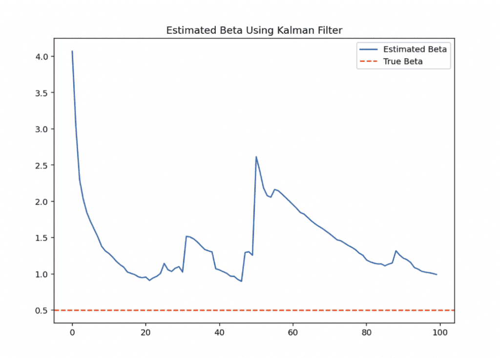
Chart

The chart below illustrates the estimated β (beta) over time using a Kalman Filter, compared to the true β value used in generating the synthetic stock data.

Initially, the estimated β starts at zero (as initialized), but as more data points are observed, the Kalman Filter dynamically adjusts and converges towards the true β.

This demonstrates the filter’s ability to update its estimates in light of new data.

This is important in pairs trading to continuously adjust the hedge ratio for market-neutral positioning.

We can also do this estimation multiple times simply by re-running the simulation with a different seed in our source code shown in the section after this (np.random.seed(X) -> change X).

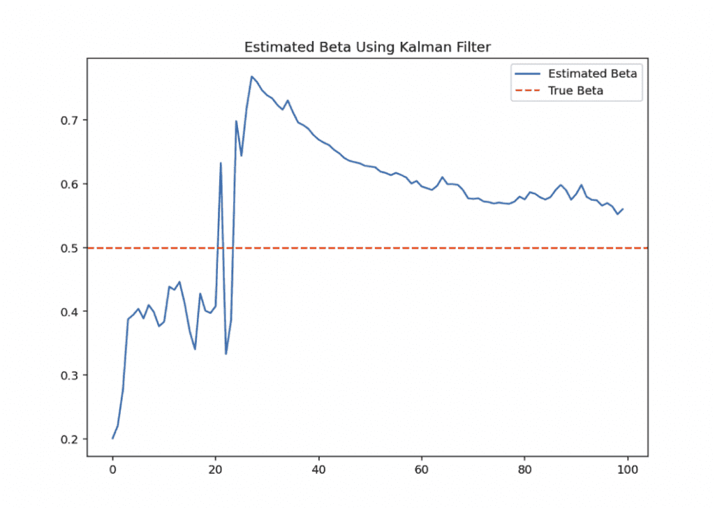
Either way, with enough trials we will hit the “long run” and see the beta estimation converge to 0.5.

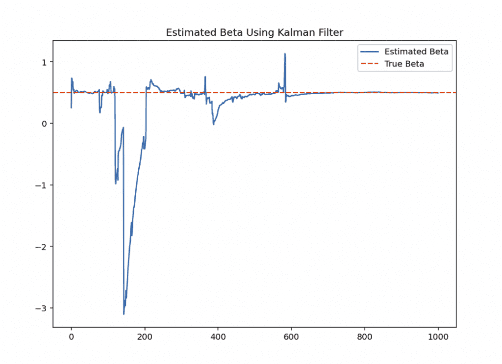
For example, we shifted the seed and did 1,000 data points instead of 100 and we can see the convergence:

Source Code in Python

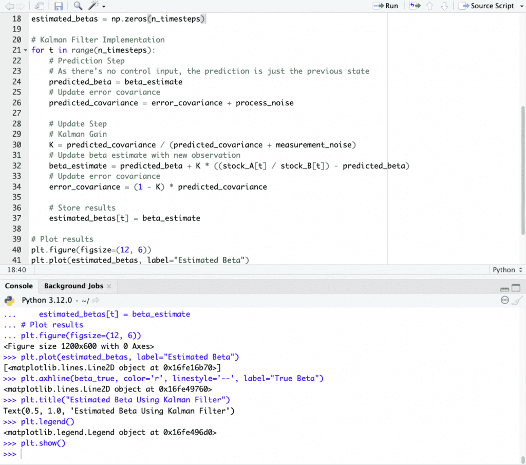
# Number of data points
n_timesteps = 100

# Synthetic stock data
np.random.seed(99)
stock_B = np.cumsum(np.random.randn(n_timesteps)) # Random walk for Stock B
beta_true = 0.5 # True beta value
stock_A = beta_true * stock_B + np.random.randn(n_timesteps) # Stock A prices with some noise

# Parameters for the Kalman Filter
beta_estimate = 0.0 # Initial estimate of beta
error_covariance = 1.0 # Initial covariance estimate
# Assume some process and measurement noise
process_noise = 0.001 # Variance in the system, small indicates we trust the model's predictions
measurement_noise = 1.0 # Variance in our observations, large indicates noisy observations

# Arrays to store the filtered results
estimated_betas = np.zeros(n_timesteps)

# Kalman Filter Implementation
for t in range(n_timesteps):
# Prediction Step
# As there's no control input, the prediction is just the previous state
predicted_beta = beta_estimate 
# Update error covariance
predicted_covariance = error_covariance + process_noise

# Update Step
# Kalman Gain
K = predicted_covariance / (predicted_covariance + measurement_noise)
# Update beta estimate with new observation
beta_estimate = predicted_beta + K * ((stock_A[t] / stock_B[t]) - predicted_beta)
# Update error covariance
error_covariance = (1 - K) * predicted_covariance

# Store results
estimated_betas[t] = beta_estimate

# Plot results
plt.figure(figsize=(12, 6))
plt.plot(estimated_betas, label="Estimated Beta")
plt.axhline(beta_true, color='r', linestyle='--', label="True Beta")
plt.title("Estimated Beta Using Kalman Filter")
plt.legend()
plt.show()

Indenting properly is important in Python, so please indent as appropriate if using this code:

FAQs – Kalman Filters

What is a Kalman Filter and how does it work?

A Kalman Filter is a recursive algorithm that estimates the state of a dynamic system from noisy observations by predicting and updating estimates with new data.

Why are Kalman Filters used in pairs trading strategies?

Kalman Filters are used in pairs trading to dynamically estimate the hedge ratio.

It adapts to changing market conditions for optimal portfolio adjustments.

What are the key components of a Kalman Filter?

The key components of a Kalman Filter include the state vector, observation matrix, transition matrix, process noise, measurement noise, and error covariance.

Each helps with the prediction and correction of the state estimate.

How do the process noise and measurement noise parameters affect the behavior of a Kalman Filter?

Process noise and measurement noise parameters in a Kalman Filter dictate the filter’s trust in the model’s predictions and the accuracy of observations.

What’s an example of a scenario in finance where Kalman Filters might be useful besides pairs trading?

We can think of a couple of examples.

Kalman Filters are useful in:

• tracking and predicting time-varying risk premiums in asset pricing (e.g., return on stocks versus the return on 10-year government bonds)
• optimizing dynamic asset allocation in portfolio management

What are some challenges or limitations of implementing Kalman Filters in real-world financial models?

Challenges of implementing Kalman Filters in finance include:

• model mis-specification
• computational intensity, and
• the need for high-frequency, accurate data

How does a Kalman Filter handle non-linear relationships in financial data?

For non-linear relationships, extensions of the basic Kalman Filter, such as the Extended Kalman Filter or Unscented Kalman Filter, are used to approximate the state estimates.

What are some common techniques to evaluate the performance of a Kalman Filter in a trading strategy?

Performance of a Kalman Filter in trading is typically evaluated through backtesting, measuring metrics like prediction accuracy, portfolio returns, and risk-adjusted performance.