9+ Volatility Models in Financial Markets

Various volatility models have been developed to understand, predict, and harness volatility.

Volatility represents the degree of variation of a financial instrument’s price over time.

While volatility is not necessarily risk itself, it’s a form of risk. So, broadly speaking, the higher the volatility, the riskier the security.

We look into some of the most prominent volatility models used.

Key Takeaways – Volatility Models in Financial Markets

• Implied Volatility (IV)
  • Derived from option’s market price, indicates future volatility expectations.
• Volatility Smile
  • Graph of implied volatility against strike prices, showing a curve.
• Volatility Clustering
  • High volatility days likely followed by high volatility days, and vice versa.
• Local Volatility
  • Volatility as a function of stock price and time.
• Stochastic Volatility
  • Assumes volatility is random and changes over time.
• Jump-Diffusion Models
  • Incorporate sudden price jumps with standard diffusion process.
• ARCH (Autoregressive Conditional Heteroskedasticity)
  • Captures volatility clustering in financial time series.
• GARCH (Generalized Autoregressive Conditional Heteroskedasticity)
  • Extends ARCH, adding lagged values of variance as variables.
• Quantum Volatility Models
  • Applying principles of quantum mechanics to better understand volatility behavior.

Implied Volatility

Implied volatility (IV) is derived from an option’s market price.

It reflects the market’s expectation of future volatility.

Unlike historical volatility which looks at past price changes, IV looks forward.

The Black-Scholes model is commonly used to compute implied volatility.

When actual option prices deviate from the Black-Scholes model’s predictions, IV can be reverse-engineered to explain the difference.

IV is a crucial metric for options traders as it can indicate whether an option is overpriced or underpriced.

Volatility Smile

The volatility smile is a phenomenon where implied volatility is plotted against strike prices.

Instead of a flat line, the graph often shows a curve resembling a smile, as shown below.

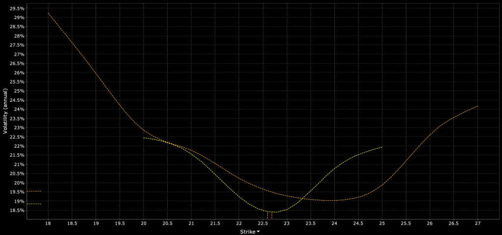
This curve indicates that out-of-the-money and in-the-money options tend to have higher implied volatilities than at-the-money options.

The volatility smile challenges the Black-Scholes model, which assumes a constant volatility.

Various factors, including supply and demand pressures, contribute to the volatility smile.

Volatility Clustering

Volatility clustering refers to the observation that high volatility days are likely to be followed by high volatility days, and low volatility days are likely to be followed by low volatility days.

This phenomenon suggests that volatility is not random but exhibits patterns.

Recognizing these patterns can be beneficial for risk management and trading strategies.

Local Volatility

Local volatility models are extensions of the Black-Scholes model.

They allow volatility to be a function of both the stock price and time.

The Dupire formula is a popular method to derive local volatility.

By using market prices of European options, one can extract a unique local volatility surface.

This model is particularly useful for pricing exotic options.

Stochastic Volatility

Stochastic volatility models assume that volatility itself is random and can change over time.

For example, the Heston model is a well-known stochastic volatility model.

In this model, volatility follows a mean-reverting square-root diffusion process.

Stochastic volatility models capture the volatility clustering phenomenon more effectively than constant volatility models.

Jump-Diffusion Models

Jump-diffusion models incorporate sudden price jumps into the standard diffusion process.

These models recognize that financial markets can experience abrupt movements due to unexpected news or events.

The Merton jump-diffusion model is a pioneering model in this category.

By adding a jump component, it provides a better fit to observed market option prices.

ARCH (Autoregressive Conditional Heteroskedasticity)

The ARCH model, introduced by Robert Engle, is designed to capture volatility clustering in financial time series.

In this model, the variance of the current period’s error term is a function of the previous periods’ squared error terms.

The ARCH model has been instrumental in modeling financial time series where volatility changes over time.

GARCH (Generalized Autoregressive Conditional Heteroskedasticity)

The GARCH model extends the ARCH model by adding lagged values of the variance itself as explanatory variables.

Introduced by Tim Bollerslev, the GARCH model is widely used in financial econometrics.

It captures both short-term and long-term effects on volatility.

The model is particularly adept at modeling and forecasting financial market volatility.

Quantum Volatility Models

Quantum volatility models use the principles of quantum mechanics to capture financial market volatility.

By harnessing the computational advantages of quantum systems, these models can process vast amounts of data and account for complex market interactions more efficiently than classical models.

Quantum models process complex data faster, capturing subtle market changes and correlations that classical models might overlook, providing deeper insights into volatility’s behavior.

FAQs – How to Model Volatility in Financial Markets

What is Implied Volatility and why is it important?

Implied Volatility (IV) is a metric derived from the current market price of a financial instrument, typically an option.

It represents the market’s expectation of how volatile the underlying asset will be over the life of the option.

IV is crucial because it helps traders assess the relative value of an option, whether it’s overpriced or underpriced, based on the market’s future volatility expectations.

What causes the Volatility Smile?

The Volatility Smile is a pattern where implied volatility is higher for options that are deep in-the-money or out-of-the-money, and lower for at-the-money options.

This phenomenon can be attributed to several factors including flows and positioning, demand and supply imbalances for particular options, and the possibility of large price jumps in the underlying asset.

What is Volatility Clustering?

Volatility Clustering refers to the observation that high volatility days in financial markets tend to be followed by high volatility days, and low volatility days tend to be followed by low volatility days.

This means that volatility is not constant over time but tends to cluster in periods.

How does Local Volatility differ from other volatility measures?

Local Volatility models the volatility of an underlying asset as a function of both time and the asset’s price.

It provides a more detailed view of volatility compared to other measures which might consider volatility as constant or time-dependent only.

Local Volatility is often used in the pricing of exotic options where standard models might not be appropriate.

What is Stochastic Volatility and how is it used in modeling?

Stochastic Volatility refers to models where volatility itself is considered a random process, subject to certain stochastic factors.

In these models, volatility can change unpredictably over time, capturing the real-world unpredictability of financial markets.

It’s used to improve option pricing accuracy, especially for longer-dated options.

How do Jump-Diffusion Models enhance volatility modeling?

Jump-Diffusion Models incorporate sudden and unexpected jumps in asset prices, in addition to the standard diffusion process.

These models recognize that financial markets can sometimes react abruptly to news or events, leading to significant price changes.

By accounting for these jumps, the models provide a more realistic representation of market behaviors.

What are ARCH and GARCH models?

ARCH (Autoregressive Conditional Heteroskedasticity) and GARCH (Generalized Autoregressive Conditional Heteroskedasticity) models are used to model and forecast volatility.

ARCH models volatility as a function of past error terms, while GARCH extends the ARCH model by including lagged values of both the error term and the variance.

They are particularly useful in capturing the volatility clustering phenomenon in financial time series data.

Why is GARCH preferred over ARCH in many applications?

ARCH provides a foundation for modeling volatility as a function of past error terms, but GARCH offers a more general approach by also considering past variances.

This makes GARCH models more flexible and better suited to capture the dynamics of financial markets, leading to their widespread preference in many financial applications.

Conclusion

Understanding and modeling volatility is important in financial markets because volatility represents one component or interpretation of risk..

The models discussed above offer a variety of options for traders, risk managers, and financial analysts.