Tail Risk Parity

Tail Risk Parity is a trading or investment strategy designed to address the asymmetrical risks inherent in financial markets.

It extends the concept of risk parity, which emphasizes an equal distribution of risk across various asset classes, by specifically focusing on mitigating the impact of extreme market movements or “tail risks.”

These tail events, though rare, can lead to significant financial losses.

Key Takeaways – Tail Risk Parity

• Risk Allocation
  • Tail Risk Parity focuses on allocating investment risks equally across various assets during extreme market conditions.
  • Rather than just targeting equal allocation of capital.
• Downside Protection
  • It aims to minimize the impact of tail events – rare but catastrophic market movements – providing better portfolio protection during crises.
• Dynamic Hedging
  • Tail Risk Parity involves dynamically adjusting portfolio hedges based on predicted tail risks.
  • Uses advanced statistical methods to predict and mitigate extreme losses.

Conceptual Framework

Origins of Risk Parity

Risk parity emerged as a response to traditional portfolio allocation methods, like the 60/40 stock/bond split.

This approach assigns weights to assets based not on their expected returns, but on their contribution to the portfolio’s overall risk.

Incorporating Tail Risk

Tail Risk Parity takes this concept further by concentrating on the tails of the distribution of returns, particularly the negative tail.

It tries to create a portfolio that is less sensitive to extreme market downturns, which are often underrepresented in standard risk models.

Methodology

Assessing Tail Risk

To implement Tail Risk Parity, investors first need to measure the tail risk associated with different assets.

This involves statistical techniques that estimate the likelihood and impact of rare, extreme market events.

Methods like Value at Risk (VaR) and Conditional Value at Risk (CVaR) are commonly used.

Portfolio Construction

In constructing a Tail Risk Parity portfolio, assets are weighted according to their tail risk contribution.

This often leads to higher allocation in assets perceived to be safer during market downturns, such as certain fixed-income securities, while reducing exposure to more volatile assets like equities.

Application in Investment Strategies

Diversification Benefits

Tail Risk Parity offers enhanced diversification benefits.

By focusing on extreme risks, it prepares the portfolio for a wider range of market scenarios, not just those within the bounds of normal market fluctuations.

Performance in Market Crises

Historically, portfolios employing Tail Risk Parity have shown resilience during market crises.

Their construction allows them to better withstand shocks that would significantly impact traditionally diversified portfolios.

Tail Risk Parity – Python Coding Example

Let’s say we wanted to adopt a relatively well-balanced but leveraged portfolio that contained the following weights relative to our capital:

• 100% Stocks: +6% forward return, 15% annualized volatility using standard deviation
• 180% Bonds: +4% forward return, 10% annualized volatility using standard deviation
• 15% Commodities: +3% forward return, 15% annualized volatility using standard deviation
• 30% Gold: +3% forward return, 15% annualized volatility using standard deviation

We can see that these notional exposures add up to 325% (3.25x leverage).

And relative to these exposures stocks make up 31% of the allocation, bonds are 55%, commodities are about 5%, and gold is about 9%.

We want to build a diagram of a Monte Carlo simulation of returns as well as a 99% VaR figure.

Here’s our code in Python for finding this:

import numpy as np

import matplotlib.pyplot as plt

# Portfolio weights are bolded

weights = np.array([1.0, 1.80, 0.15, 0.3])

# Expected forward returns

returns = np.array([0.06, 0.04, 0.03, 0.03])

# Annualized volatility (standard deviation)

volatility = np.array([0.15, 0.10, 0.15, 0.15])

# Correlation matrix (0% correlation between assets)

correlation_matrix = np.eye(4)  # Identity matrix for 0% correlation

# Number of sims

num_simulations = 10000

# Time horizon in yrs for the simulation

time_horizon = 1

# Convert the correlation matrix to a covariance matrix

cov_matrix = np.outer(volatility, volatility) * correlation_matrix

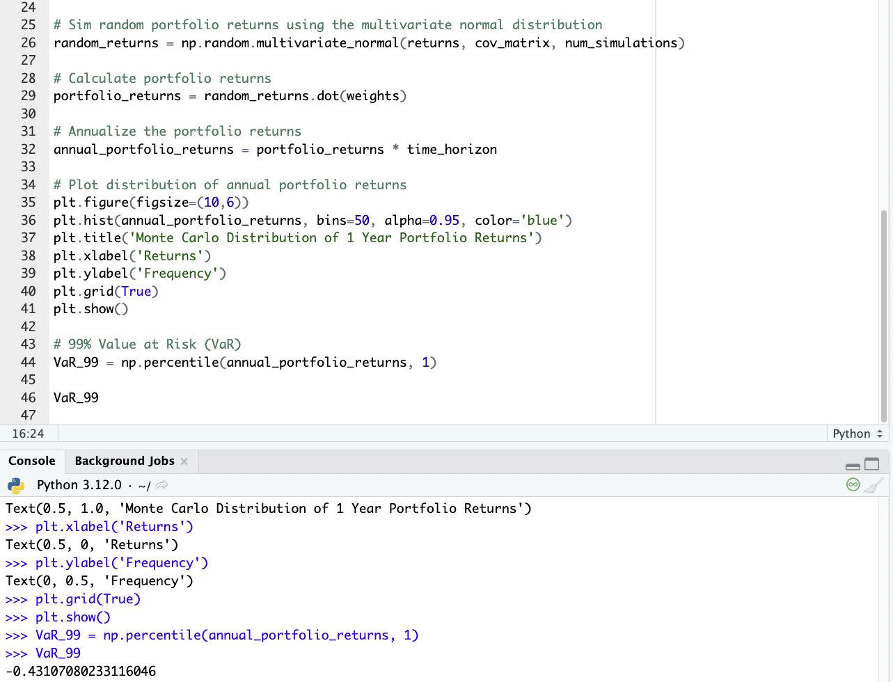
# Sim random portfolio returns using the multivariate normal distribution

random_returns = np.random.multivariate_normal(returns, cov_matrix, num_simulations)

# Calculate portfolio returns

portfolio_returns = random_returns.dot(weights)

# Annualize the portfolio returns

annual_portfolio_returns = portfolio_returns * time_horizon

# Plot distribution of annual portfolio returns

plt.figure(figsize=(10,6))

plt.hist(annual_portfolio_returns, bins=50, alpha=0.95, color='blue')

plt.title('Monte Carlo Distribution of 1 Year Portfolio Returns')

plt.xlabel('Returns')

plt.ylabel('Frequency')

plt.grid(True)

plt.show()

# 99% Value at Risk (VaR)

VaR_99 = np.percentile(annual_portfolio_returns, 1)

VaR_99

Here’s our diagram of returns:

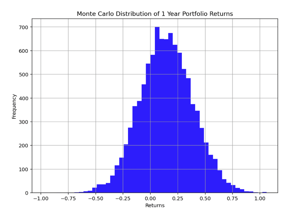
And our 99% VaR comes out to about 43.1%.

In other words, in the worst 1% of circumstances, our loss comes to 43.1%.

For traders or portfolio managers uncomfortable with this figure, they would generally use options to remove left-tail risk, take less risk, or figure out ways to diversify better to change the nature of the distribution.

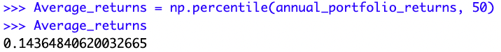
Average Returns

How about average returns?

We can add in these lines:

Average_returns = np.percentile(annual_portfolio_returns, 50) 

Average_returns

And we get 14.3%.

Challenges and Limitations

Complexity of Implementation

Implementing Tail Risk Parity is complex.

It requires sophisticated risk modeling capabilities and a deep understanding of the statistical properties of asset returns, especially in the tails of the distribution.

Dynamic Market Conditions

The strategy also needs to be adaptive to changing market conditions.

Tail risks can evolve over time, and the portfolio must be regularly reassessed and rebalanced accordingly.

Conclusion

Tail Risk Parity is part of a broader class of risk-focused investment strategies.

By specifically addressing the risk of extreme market events, it offers a framework for portfolio construction that can enhance resilience in times of market stress.

Nevertheless, its successful implementation demands statistical analysis and a proactive approach to portfolio management.