Bayesian Methods in Finance


Bayesian analysis in finance, trading, and investing is a framework that incorporates probabilistic modeling and decision-making under uncertainty.
This approach is based on Bayesian inference, where prior beliefs are updated with new information to form posterior beliefs.
Key Takeaways – Bayesian Methods in Finance
- Bayesian methods in finance offer a probabilistic framework for incorporating prior knowledge and real-time data to model uncertainty and make informed decisions.
- Applications include risk management, portfolio optimization, and asset valuation.
- Non-parametric Bayesian methods are capable of capturing complex patterns and relationships in data without being constrained by the rigid structures of parametric models.
- Their adaptability and ability to incorporate prior knowledge make them particularly suitable for financial markets.
- Variational Bayesian methods in finance enable the application of Bayesian models to complex, high-dimensional problems where traditional methods may be computationally prohibitive.
- By providing faster and scalable inference, they are particularly useful in areas requiring real-time analysis or handling large-scale financial data.
Key Concepts in Bayesian Analysis in Finance
Let’s explore the key concepts:
Bayesian Inference
This is the process of updating the probability estimate for a hypothesis as more evidence or information becomes available.
It’s central to Bayesian analysis in finance, where market information is continuously incorporated into models.
A common example would be integrating information from an earnings announcement into a stock price.
Earnings updates an existing view of a company, its finances, where it’s going, and what that means for its stock.
Bayesian Probability
Unlike frequentist probability, which interprets probability as the long-run frequency of events, Bayesian probability is a measure of the degree of belief or confidence in the occurrence of an event.
Bayes’ Theorem
This theorem describes how to update the probabilities of hypotheses when given evidence.
It’s fundamental in Bayesian analysis for revising beliefs in the light of new data.
Bernstein–von Mises Theorem
This theorem provides a justification for Bayesian methods from a frequentist perspective, showing that under certain conditions, the Bayesian posterior distribution converges to a normal distribution centered around the true parameter value as sample size increases.
Coherence
In Bayesian analysis, coherence refers to the internal consistency of a set of probability assignments.
A coherent set of probabilities doesn’t contain any contradictions.
Cox’s Theorem
This theorem underpins the foundations of Bayesian probability theory, showing that Bayesian updating follows logically from certain consistency axioms.
In finance, e.g., a stock reacts in predictable ways to an earnings announcement based on how results are relative to discounted expectations.
Cromwell’s Rule
In Bayesian analysis, this rule advises against assigning a probability of 0 or 1 to an event unless it is logically certain.
It acknowledges the need to keep an open mind to new evidence.
A problem with traders is they often become overconfident when markets are ultimately a game of probabilities.
This is why the future outcomes of the assets one trades are commonly represented analytically as distributions, such as the following:
Related: Psychological Biases and How to Avoid Them
Principle of Indifference
This principle suggests assigning equal probabilities to all outcomes when no additional information is available.
For example, if you have a choice between Stock A and Stock B and haven’t studied either company, then betting on one over the other probably doesn’t make sense.
Principle of Maximum Entropy
When choosing a probability distribution, one should pick the distribution with the maximum entropy consistent with the given constraints, to make the least biased estimate possible.
Model Building
In finance, Bayesian model building involves specifying a prior distribution and a likelihood function, from which the posterior distribution is derived.
Weak Prior … Strong Prior
- A weak (or non-informative) prior reflects a lack of prior knowledge.
- A strong prior is based on substantial prior knowledge or strong beliefs about the parameters.
Conjugate Prior
A conjugate prior is chosen because its form simplifies the analytical computation of the posterior distribution.
Linear Regression
Bayesian linear regression uses Bayes’ theorem for regression analysis, providing probabilistic interpretations of model parameters and predictions.
Empirical Bayes
This method estimates prior distributions from the data.
Combines the ideas of both frequentist and Bayesian statistics.
Hierarchical Model
This involves structuring parameters into layers, with each layer being conditional on parameters from the higher layer, useful for handling complex data structures in finance.
Example of a Hierarchical Model in Finance
In a hierarchical Bayesian model applied to finance, one might structure the model such that individual asset returns are conditioned on sector-specific parameters, which in turn are conditioned on broader market parameters.
For example, if the S&P 500 goes up +1% in a day based on a certain drop in interest rates, we might assume that the energy sector would perform similarly.
This allows for nuanced analysis that captures both micro-level asset behaviors and macro-level market trends.
This layered approach facilitates the modeling of complex dependencies and interactions within financial datasets.
This offers a more detailed and interconnected understanding of risk and return dynamics across different levels of a certain financial market.
Posterior Approximation
Techniques like Markov chain Monte Carlo (MCMC), Laplace’s approximation, Integrated nested Laplace approximations, and Variational inference are used for approximating complex posterior distributions that are difficult to compute analytically.
Markov Chain Monte Carlo (MCMC)
A computational technique that uses random sampling to approximate complex and high-dimensional posterior distributions in Bayesian inference.
Laplace’s Approximation
A method that approximates a complex posterior distribution by a Gaussian distribution centered at the mode of the posterior.
Integrated Nested Laplace Approximations (INLA)
A technique for approximate Bayesian inference in latent Gaussian models, offering faster computations than MCMC.
Variational Inference
An optimization-based approach that approximates complex posterior distributions by simpler, parameterized distributions to make Bayesian inference computationally tractable.
Estimators
In Bayesian analysis, estimators are used to summarize the posterior distribution, such as the Bayesian estimator and Maximum a posteriori estimation.
Credible Interval
This is the Bayesian equivalent of confidence intervals, representing the range within which an unobserved parameter lies with a certain probability.
Evidence Approximation and Evidence Lower Bound
These are methods used in Bayesian model selection and for approximating the evidence in favor of a model.
Nested Sampling
A technique used for Bayesian computation, particularly for model evidence calculation.
Model Evaluation
In Bayesian analysis, model evaluation is critical.
Bayes factor, Model averaging, and Posterior predictive checks are tools for assessing the fit and predictive accuracy of Bayesian models.
Summary
In financial contexts, these concepts are important for developing models that adapt to new information, manage risk, and make predictions.
Bayesian methods allow for a more nuanced and flexible approach to modeling financial markets, accounting for the dynamic nature of financial data.
Bayesian analysis offers a framework for addressing unknowns and incorporating subjective beliefs in finance.
Applications of Bayesian Analysis
Its applications in portfolio construction, valuation, and risk management are substantial.
Portfolio Construction
Incorporating Views and Uncertainties
Bayesian methods allow the integration of subjective views (from market experts, for instance) with historical data.
Dynamic Asset Allocation
Bayesian techniques enable dynamic updating of asset allocation as new data becomes available, helping in adapting to market changes.
Modeling Returns
Bayesian models, such as Bayesian regression, can be used to model asset returns.
Tailoring to Investor Preferences
Through Bayesian methods, portfolios can be tailored to individual risk preferences and investment horizons.
This considers the uncertainty in estimates of returns and risks.
Valuation
Estimating Cash Flows and Discount Rates
Bayesian models can provide a probabilistic approach to estimate future cash flows and discount rates.
Real Options Valuation
Bayesian analysis aids in valuing real options, where the decision-making is sequential and information is revealed over time.
Mergers and Acquisitions
In M&A scenarios, Bayesian methods can be used to incorporate information from various sources to value target companies under uncertainty.
Startup Valuation
Startups often lack historical data. Bayesian analysis helps in combining market data with expert opinions to estimate their value.
Risk Management
Credit Risk Modeling
Bayesian techniques allow for the incorporation of prior knowledge and expert opinions into credit risk models, which is especially useful when historical data is scarce or non-representative.
Market Risk Assessment
In market risk, Bayesian methods help in dynamically updating the distribution of asset returns, leading to more accurate Value at Risk (VaR) or Expected Shortfall (ES) calculations.
Operational Risk
For operational risk, which often lacks sufficient historical data, Bayesian approaches can combine internal data, external data, and expert judgment.
Stress Testing and Scenario Analysis
Bayesian models can be used to generate and update scenarios for stress testing, taking into account current market conditions and forward-looking information.
Liquidity Risk
Bayesian networks can model the dependencies between various market factors and liquidity risk, providing insights into the likelihood of liquidity crises under different scenarios.
Summary
In each of these areas, Bayesian analysis enhances the traditional methods by incorporating a level of probabilistic reasoning and dealing with unknowns in a more explicit manner.
It allows financial analysts and decision-makers to quantify their confidence in various assumptions and outcomes.
Variational Bayesian Methods in Finance
Variational Bayesian methods provide an alternative to traditional Markov Chain Monte Carlo (MCMC) techniques for approximating posterior distributions in Bayesian inference – useful in finance where models often involve complex, high-dimensional data.
These methods turn the problem of Bayesian inference into an optimization problem. This provides computational efficiency and scalability.
Key Concepts and Techniques
Variational Inference (VI)
VI approximates the posterior distribution by a simpler distribution.
It optimizes the parameters of this simpler distribution to be as close as possible to the true posterior.
Mean-Field Approximation
A common approach in VI where the joint distribution is approximated by a product of independent distributions, simplifying computations.
Evidence Lower Bound (ELBO)
In VI, the optimization involves maximizing the ELBO, which is a lower bound on the model evidence (or marginal likelihood).
Stochastic Variational Inference (SVI)
SVI combines VI with stochastic optimization.
This makes it feasible to handle large datasets often encountered in finance.
Applications in Finance
Risk Management
Variational methods can efficiently estimate the posterior distributions of risk models, such as Value at Risk (VaR) models – especially when dealing with large portfolios or complex asset dynamics.
Portfolio Optimization
In Bayesian portfolio optimization, variational methods can handle complex models, such as those incorporating investor beliefs and market views, more efficiently than MCMC.
Asset Pricing Models
Estimating parameters of sophisticated asset pricing models – especially those with a large number of latent variables or factors – can be more computationally efficient with variational methods.
Algorithmic Trading
For high-frequency trading strategies, where speed is the top factor, variational methods offer faster inference compared to traditional Bayesian methods.
This allows for real-time updating of trading models.
Credit Risk Modeling
In modeling credit risk, especially with large portfolios or complex correlation structures, variational Bayesian methods provide a scalable solution for estimating default probabilities and loss distributions.
Macroeconomic Forecasting
They are used in dynamic stochastic general equilibrium (DSGE) models and other complex macroeconomic models for faster inference and prediction.
Time-Series Analysis
Variational methods are suitable for Bayesian time-series analysis, including state-space models and dynamic linear models.
Provides quicker updates and forecasts.
Bayesian Neural Networks
In applying neural networks to financial modeling, variational Bayesian methods offer a way to quantify uncertainty in predictions.
Summary
Variational Bayesian methods in finance enable the application of Bayesian models to complex, high-dimensional problems where traditional methods may be computationally prohibitive.
By providing faster and scalable inference, they are particularly useful in areas requiring real-time analysis or handling large-scale financial data.
Their ability to quantify unknowns and incorporate prior knowledge continues to make them an increasingly popular choice in various financial applications.
Non-Parametric Bayesian Methods in Finance
Non-parametric Bayesian methods in finance are valuable for their flexibility in modeling complex and dynamic financial data without assuming a specific parametric form.
These methods adapt to the data’s structure.
This makes them well-suited for the often non-linear and non-normal/fat-tailed characteristics of financial markets.
Key applications and techniques include:
Key Techniques
Dirichlet Process (DP)
The DP is a common non-parametric Bayesian method used for clustering or modeling mixture distributions without pre-specifying the number of clusters or mixture components.
It’s useful in finance for modeling distributions of returns, identifying regimes in financial time series, or clustering assets.
Gaussian Processes (GP)
GPs are used for regression and classification tasks – offering a flexible approach to modeling unknown functions.
In finance, they’re applied for time-series forecasting, yield curve modeling, and risk management.
Bayesian Nonparametric Regression
This approach extends traditional regression models by allowing for an infinite number of parameters.
It’s useful for complex relationships in financial data, such as the relationship between macroeconomic variables and asset prices.
Infinite Hidden Markov Models (iHMM)
In iHMMs, the number of latent states is not fixed, allowing for more flexible modeling of time series with changing regimes or behaviors, such as volatility clustering in asset returns.
Applications in Finance
Risk Management
Non-parametric Bayesian methods can model the distribution of asset returns or losses more accurately, capturing fat tails and skewness often observed in financial markets.
Asset Pricing and Portfolio Allocation
These methods allow for more flexible modeling of asset return dynamics and correlations.
This aids in more robust portfolio construction and asset pricing models.
Algorithmic Trading
In algorithmic trading, non-parametric models can adapt to new market conditions more effectively – capturing complex patterns in high-frequency data for trading strategies.
Credit Scoring and Default Prediction
They can be used to model the probability of default without assuming a specific distributional form, potentially improving the accuracy of credit risk models.
Yield Curve Modeling
Non-parametric methods allow for flexible modeling of the yield curve.
Macroeconomic Forecasting
These methods provide a way to forecast economic indicators without imposing restrictive assumptions about the underlying economic relationships.
Modeling Illiquid Assets
For assets with sparse data, such as certain fixed-income securities or real estate, non-parametric Bayesian models can leverage their flexibility to provide better estimates of value and risk.
Related: Non-Parametric Models in Finance
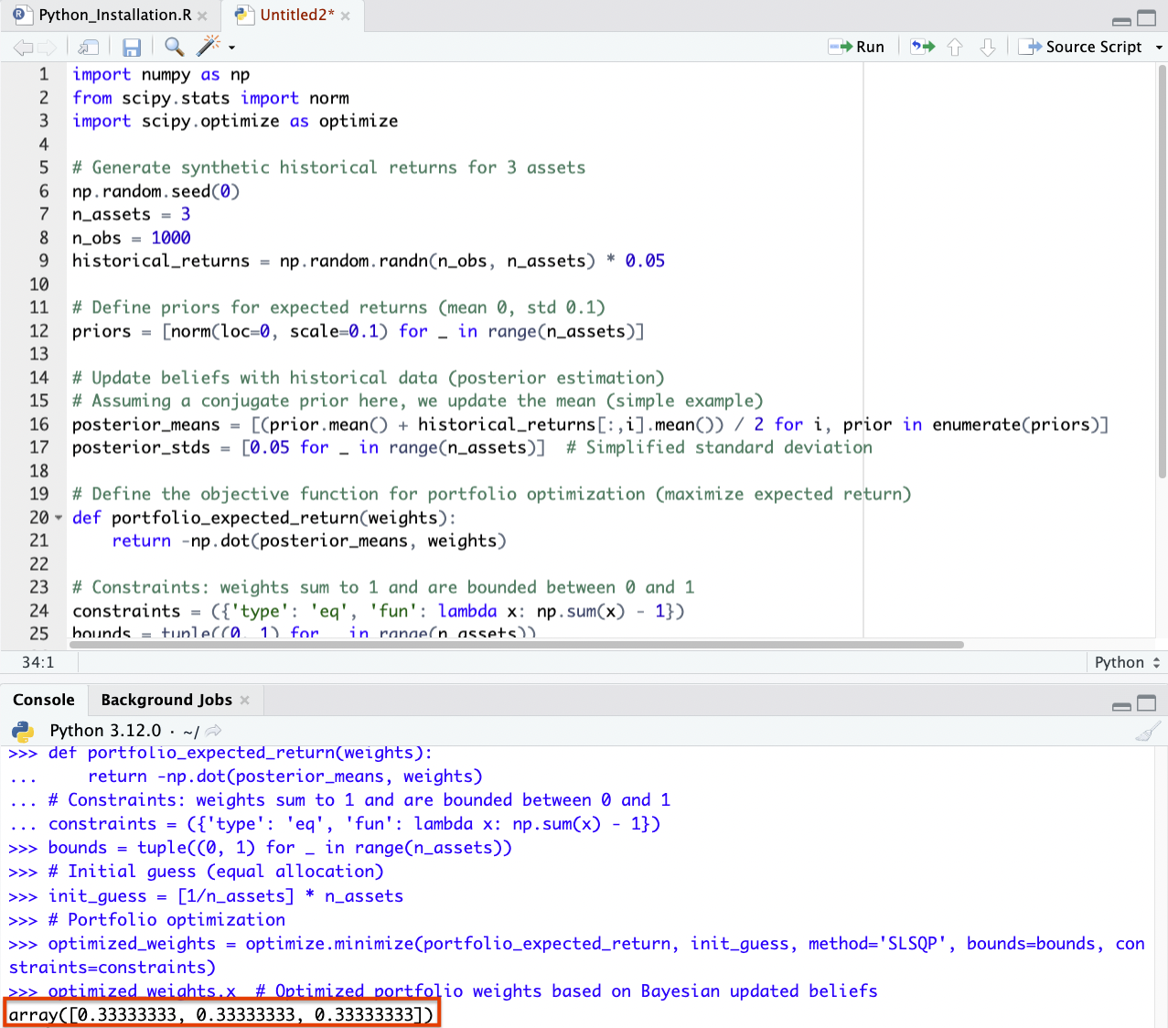
Coding Example – Bayesian Methods for Portfolio Optimization
To demonstrate a coding example for Bayesian methods in portfolio optimization, we’ll use a simplified scenario.
We’ll assume a portfolio with a few assets and use historical returns to update our beliefs about the expected returns of these assets.
For simplicity, let’s use synthetic data.
The code will follow these steps:
- Generate synthetic historical returns for a few assets.
- Define a prior distribution for expected returns (e.g., a normal distribution).
- Update the distribution with the synthetic data using Bayesian inference.
- Optimize the portfolio based on the updated beliefs about expected returns.
We’ll use Python libraries like numpy for numerical operations and scipy for statistical functions.
import numpy as np
from scipy.stats import norm
import scipy.optimize as optimize

# Generate synthetic historical returns for 3 assets
np.random.seed(0)
n_assets = 3
n_obs = 1000
historical_returns = np.random.randn(n_obs, n_assets) * 0.05

# Define priors for expected returns (mean 0, std 0.1)
priors = [norm(loc=0, scale=0.1) for _ in range(n_assets)]

# Update beliefs with historical data (posterior estimation)
# Assuming a conjugate prior here, we update the mean (simple example)
posterior_means = [(prior.mean() + historical_returns[:,i].mean()) / 2 for i, prior in enumerate(priors)]
posterior_stds = [0.05 for _ in range(n_assets)] # Simplified standard deviation

# Define the objective function for portfolio optimization (maximize expected return)
def portfolio_expected_return(weights):
return -np.dot(posterior_means, weights)

# Constraints: weights sum to 1 and are bounded between 0 and 1
constraints = ({'type': 'eq', 'fun': lambda x: np.sum(x) - 1})
bounds = tuple((0, 1) for _ in range(n_assets))

# Initial guess (equal allocation)
init_guess = [1/n_assets] * n_assets

# Portfolio optimization
optimized_weights = optimize.minimize(portfolio_expected_return, init_guess, method='SLSQP', bounds=bounds, constraints=constraints)

optimized_weights.x # Optimized portfolio weights based on Bayesian updated beliefs
In this Python example, we generated synthetic historical returns for three assets and used a simple Bayesian update mechanism to estimate the posterior expected returns.
The prior distribution for each asset’s expected return was assumed to be a normal distribution with a mean of 0 and a standard deviation of 0.1.
The posterior means were estimated by averaging the prior mean and the sample mean of the synthetic data.
For portfolio optimization, the goal was to maximize the expected return, which is the negative of the dot product of the posterior means and the portfolio weights.
The optimization was subject to the constraints that all weights sum to 1 and each weight is between 0 and 1.
The result of the optimization suggests an equal allocation across all three assets, which is the outcome of the simplistic assumptions and synthetic data used.