How to Make a Monte Carlo Simulation in Python (Finance)


Monte Carlo simulations are a tool in finance for modeling and understanding the behavior of financial systems under various scenarios.
These simulations use randomness to solve problems that might be deterministic in principle.
Python, with its rich library ecosystem, offers an efficient platform for conducting Monte Carlo simulations.
Here’s a guide on how to implement a Monte Carlo simulation in Python for financial applications.
We also have written a guide on Monte Carlo simulations for R in a separate article (as well as one related to options).
Understanding the Basics
Before diving into coding, it’s important to grasp what Monte Carlo simulations are.
In finance, these simulations are used to model the probability of different outcomes in a process that cannot easily be predicted due to the intervention of random variables.
They are particularly useful for assessing risk and uncertainty in financial forecasts and investment portfolios.
Setting Up Your Python Environment
To start, ensure you have Python installed on your system.
You will also need libraries like NumPy and Matplotlib, which can be installed via pip:
pip install numpy matplotlib
Step-by-Step Implementation
Define the Problem
Clearly outline the financial problem you wish to solve.
For instance, predicting future stock prices or assessing the risk in a portfolio.
Import Necessary Libraries
import numpy as np
import matplotlib.pyplot as plt
Related: How to Set Up Python in R Studio
Set Up the Parameters
Define the variables of your simulation.
In a stock price simulation, these might include the initial stock price, the expected return, the volatility, and the time horizon.
Generate Random Variables
Use NumPy to generate random variables that represent the uncertainty in your model.
For stock prices, these could be the daily returns:
daily_returns = np.random.normal(avg_daily_return, std_deviation, number_of_days)
Run the Simulation
Iterate the process for as many simulations as you need.
Each iteration represents a possible future scenario:
for i in range(number_of_simulations):
# Simulate the stock price and add it to the list
Analyze the Results
Once you have the simulation data, you can analyze it to draw conclusions.
This might include plotting a histogram of the final stock prices or calculating the Value at Risk (VaR).
Visualization
Use Matplotlib to visualize the results. This can help in understanding the distribution of outcomes:
plt.hist(final_prices, bins=50)
plt.show()
Example #1 – Monte Carlo in Python: Portfolio Value Simulation
Let’s consider a simple portfolio and forecast its value over a year with a Monte Carlo simulation:
- Portfolio includes different assets with specified expected returns and volatilities.
- Assume the assets are not correlated.
- Use NumPy to generate random returns for each asset.
- Calculate the portfolio value at the end of the year for each simulation.
- Plot the distribution of the final portfolio values.
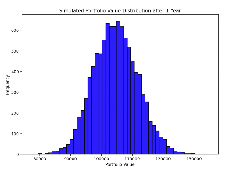
The Monte Carlo simulation code successfully forward tests the specified portfolio’s distribution over one year.
The portfolio comprises Stocks, Bonds, Cash, and Gold, each with its own allocation, expected return, and volatility:
Portfolio Composition
- Stocks (35% allocation, 6% return, 15% volatility)
- Bonds (40% allocation, 4% return, 10% volatility)
- Cash (10% allocation, 3% return, 0% volatility)
- Gold (15% allocation, 3% return, 15% volatility)
Simulation Parameters
The simulation runs 10,000 iterations – which is standard – covering a broad spectrum of potential outcomes.
The time horizon is one year, with an initial investment of $100,000.
Simulation Process
Each iteration calculates the final portfolio value by applying the return and volatility for each asset class, considering their specific allocations.
The assets are assumed to be uncorrelated.
Results Visualization
The histogram shows the distribution of final portfolio values across all simulations.
This distribution offers insights into the potential range and likelihood of different portfolio outcomes after one year, given the defined asset allocation and market conditions.
In short, this Monte Carlo simulation provides a visual and quantitative understanding of the risks and potential returns associated with a specific portfolio configuration.
import numpy as np
import matplotlib.pyplot as plt

# Monte Carlo simulation for forward testing a specific portfolio's distribution over one year

# Portfolio composition with allocations, expected returns, and volatilities
portfolio = {
"Stocks": {"allocation": 0.35, "return": 0.06, "volatility": 0.15},
"Bonds": {"allocation": 0.40, "return": 0.04, "volatility": 0.10},
"Cash": {"allocation": 0.10, "return": 0.03, "volatility": 0},
"Gold": {"allocation": 0.15, "return": 0.03, "volatility": 0.15}
}

# Simulation parameters
num_simulations = 10000 # Number of Monte Carlo simulations
time_horizon = 1 # Time horizon for the simulation (1 year)
initial_investment = 100000 # Initial investment amount

# Simulating portfolio value over the time horizon
portfolio_values = np.zeros(num_simulations)
np.random.seed(0) # For reproducibility

for i in range(num_simulations):
final_value = initial_investment

# Calculating portfolio value at the end of time horizon for each asset
for asset, info in portfolio.items():
annual_return = info["return"]
annual_volatility = info["volatility"]
random_return = np.random.normal(annual_return, annual_volatility)
final_value += final_value * info["allocation"] * random_return

portfolio_values[i] = final_value

# Plotting the distribution of portfolio values with adjusted scale
plt.hist(portfolio_values, bins=50, color='blue', edgecolor='black')
plt.title('Simulated Portfolio Value Distribution after 1 Year')
plt.xlabel('Portfolio Value')
plt.ylabel('Frequency')
plt.show()
Be sure to indent the code as needed:
Below is a histogram of returns (100,000 is the center point):
Example #2 – Monte Carlo in Python: Portfolio VaR
We take the same Monte Carlo simulation as above and estimate the risk of a portfolio – specifically calculating the Value at Risk (VaR) and Conditional Value at Risk (CVaR) over one year:
Portfolio Composition
The simulation considered a portfolio consisting of Stocks, Bonds, Cash, and Gold, each with specified allocations, returns, and volatilities.
Simulation Details
10,000 simulations were performed over a one-year time horizon, starting with an initial investment of $100,000.
VaR and CVaR Calculation
Value at Risk (VaR)
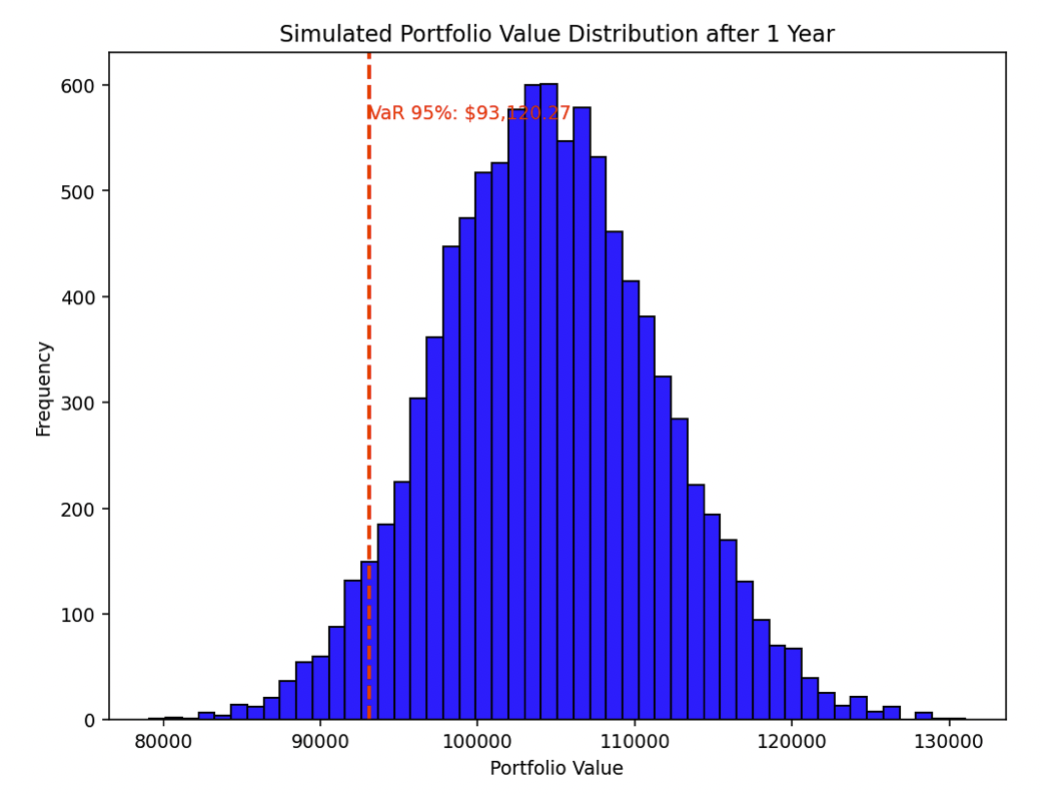
The VaR at a 95% confidence level was calculated, which represents the minimum loss expected over the time horizon in the worst 5% of cases.
The VaR for this portfolio is approximately $92,995.54.
Conditional Value at Risk (CVaR)
CVaR provides the expected loss in the worst 5% of cases.
The CVaR for this portfolio is approximately $90,198.65.
When we run this in our IDE, we see values similar to each (they’ll vary slightly by simulation):
Result Interpretation
The VaR and CVaR provide insights into the potential risk of the portfolio.
A lower VaR and CVaR indicate lower risk.
Visualization
The histogram visualizes the distribution of portfolio values after one year.
The red dashed line represents the VaR, indicating where the lower 5% of the distribution begins.
This analysis is useful for understanding the risk profile of a portfolio, helping traders/investors make informed decisions about risk management and trading/investment strategies.
It can be viewed below:
And the source code:
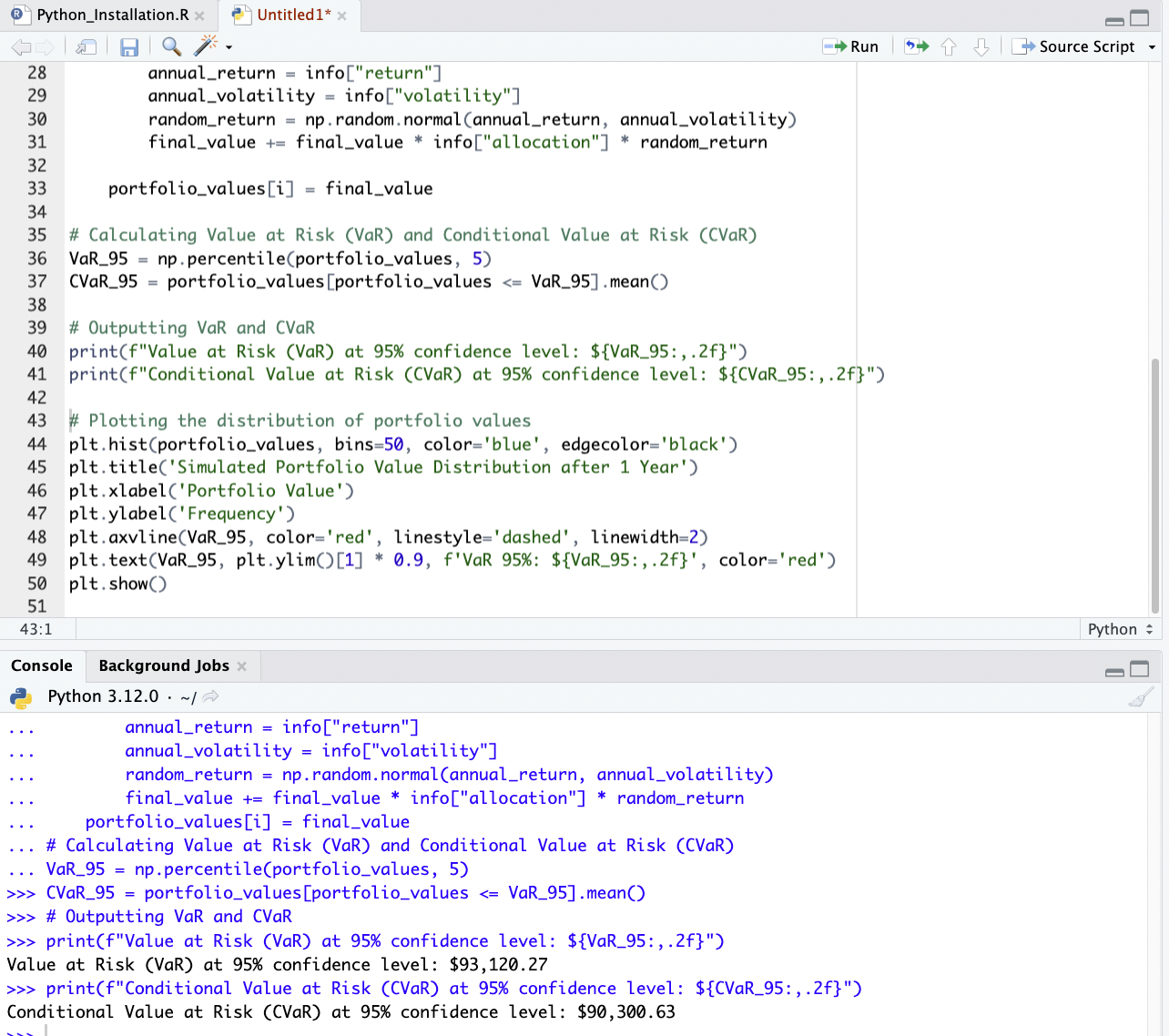
import numpy as np
import matplotlib.pyplot as plt

# Monte Carlo simulation for forward testing a specific portfolio's distribution over one year

# Portfolio composition with allocations, expected returns, and volatilities
portfolio = {
"Stocks": {"allocation": 0.35, "return": 0.06, "volatility": 0.15},
"Bonds": {"allocation": 0.40, "return": 0.04, "volatility": 0.10},
"Cash": {"allocation": 0.10, "return": 0.03, "volatility": 0},
"Gold": {"allocation": 0.15, "return": 0.03, "volatility": 0.15}
}

# Simulation parameters
num_simulations = 10000 # Number of Monte Carlo simulations
time_horizon = 1 # Time horizon for the simulation (1 year)
initial_investment = 100000 # Initial investment amount

# Simulating portfolio value over the time horizon
portfolio_values = np.zeros(num_simulations)
np.random.seed(0) # For reproducibility

for i in range(num_simulations):
final_value = initial_investment

# Calculating portfolio value at the end of time horizon for each asset
for asset, info in portfolio.items():
annual_return = info["return"]
annual_volatility = info["volatility"]
random_return = np.random.normal(annual_return, annual_volatility)
final_value += final_value * info["allocation"] * random_return

portfolio_values[i] = final_value

# Calculating Value at Risk (VaR) and Conditional Value at Risk (CVaR)
VaR_95 = np.percentile(portfolio_values, 5)
CVaR_95 = portfolio_values[portfolio_values <= VaR_95].mean()

# Outputting VaR and CVaR
print(f"Value at Risk (VaR) at 95% confidence level: ${VaR_95:,.2f}")
print(f"Conditional Value at Risk (CVaR) at 95% confidence level: ${CVaR_95:,.2f}")

# Plotting the distribution of portfolio values
plt.hist(portfolio_values, bins=50, color='blue', edgecolor='black')
plt.title('Simulated Portfolio Value Distribution after 1 Year')
plt.xlabel('Portfolio Value')
plt.ylabel('Frequency')
plt.axvline(VaR_95, color='red', linestyle='dashed', linewidth=2)
plt.text(VaR_95, plt.ylim()[1] * 0.9, f'VaR 95%: ${VaR_95:,.2f}', color='red')
plt.show()
Best Practices and Considerations
Quality of Random Numbers
Ensure that the random number generator is suitable for your application.
NumPy’s random module is generally sufficient for basic simulations.
Number of Simulations
More simulations generally provide more accurate results, but also require more computational power.
10,000 is a popular number used for many types of simulations to help fill out a distribution.
But it depends on what you’re trying to do.
Model Assumptions
Be aware of the assumptions in your model.
Monte Carlo simulations are only as good as the models and assumptions they are based on.
What Are Some Different Types of Monte Carlo Simulations You Can Do in Python?
Some different models you can do:
Stock Price Forecasting
Simulating future stock prices using models like the Geometric Brownian Motion.
Portfolio Risk Analysis
Estimating the risk of a portfolio.
Like calculating the Value at Risk (VaR) or Conditional Value at Risk (CVaR).
Option Pricing
Using models like the Black-Scholes model to simulate the pricing of options under various market conditions.
Credit Risk Modeling
Simulating the likelihood of credit default and the loss distribution for credit portfolios.
Interest Rate Modeling
Simulating future interest rate movements to assess the interest rate risk in a bond portfolio.
Asset Allocation
Testing different portfolio compositions to determine optimal asset allocation strategies.
Real Options Analysis
Evaluating investment decisions under uncertainty, like in capital budgeting.
Economic Forecasting
Simulating macroeconomic variables to predict future economic scenarios and their impact on asset prices (and other financial variables).
Derivative Valuation
Assessing the value of complex financial derivatives under various market scenarios.
Liquidity Risk Analysis
Estimating the impact of liquidity constraints on asset prices and portfolio values.
Cash Flow Modeling
Projecting future cash flows for businesses or investment projects under different scenarios.
Project Risk Management
Assessing the risk and return of projects or business ventures by simulating various outcomes and unknowns.
Conclusion
Monte Carlo simulations in Python offer a versatile way to model financial scenarios with inherent unknowns.
By carefully setting up the simulation parameters and critically analyzing the results, you can gain insights into the financial models and trading/investment strategies.