Monte Carlo Simulations of Options Pricing Models in R

Monte Carlo simulation is a useful tool for simulating a variety of financial events, including options pricing models.

Naturally, finance and investing is a world of uncertainty, so modeling situations mathematically and simulating them through thousands of iterations is of interest in order to forecast how the situation might play out.

Ultimately, it can help the trader or investor determine whether he or she is making a prudent financial decision based on the input parameters.

There is always the ability to model financial events in software such as Excel, SAS, and R, but writing something from scratch requires a large degree of coding knowledge in order to appropriately formulate the model.

Sometimes this is inevitable, although once you get over the learning curve it should be a breeze.

But in the meantime, we’re going to show you an installation package that can be installed in R in order to quickly and efficiently create a variety of Monte Carlo options pricing models with a fraction of the coding.

The mathematical technique integrated into this package involves the Least Squares Monte Carlo method, which allows for accurate valuation of options where other mathematical techniques like finite differences and binomial approaches fail when multiple valuation factors are involved.

All that is required is some basic code inputs and you will be set to simulate a variety of different situations.

What you will need

First, you need R and R Studio in order to set this up. There are various tutorial videos online (e.g., YouTube) should you need assistance with the initial setup.

The required package is called LSMonteCarlo, which can be completed by clicking on the packages tab in the interface, then “Install” and typing in “LSMonteCarlo” as is.

Before using, “LSMonteCarlo” must be checked in the “Packages” tab to get it up and running for use.

Overview of LSMonteCarlo

LSMonteCarlo is comprised of functions for calculating the prices of American put options via the Least Squares Monte Carlo method.

The package includes a variety of option types and calculating functions, including:

• American put
• Asian American put
• Quanto American put
• European put (with Black-Scholes analytical solution)
• European call (ditto)
• Pricing algorithms for variance reduction including Antithetic Variates (AV) and Control Variates
• Geometric Brownian motion generation
• 3D plotting capacity of the relationship between options prices based on their corresponding volatility and strike price parameters

Function Examples

I’ve outlined the following nine functions that I have found of great use when calculating option premium prices.

For reference, the variables featured in this function include the following:

• Spot: Current price of the underlying asset (i.e., stock)
• vols: Volatility sequence
• n: Number of simulated paths (i.e., number of iterations simulated)
• m: Number of simulated time steps in each path/iteration
• r: Interest rate in the currency being used to purchase the option
• dr: Dividend rate of the underlying asset
• mT: Maturity time in years
• rho: Correlation coefficient between two options (to be used for Quanto American options)

Note: number of data points for each simulation matrix will be n * m

#1

This code will provide the option price at a variety of different volatilities and strike prices.

plot(AmerPutLSMPriceSurf(vols = (seq(0.1, 1.5, 0.2)), n=200, m=10,
strikes = (seq(0.5, 1.9, 0.2))), color = divPalette(150, "RdBu"))

Volatilities and strikes are specified in the seq() parenthetical.

For instance, in the volatility part of the code (“vols=”), 0.1 denotes the lower bound volatility, 1.5 specifies the upper bound, and 0.2 states the increment.

Hence this function will calculate prices for volatilities of 0.1, 0.3, 0.5, 0.7, 0.9, 1.1, 1.3, and 1.5. The strikes, based on the set parameters, would be 0.5, 0.7, 0.9, 1.1, 1.3, 1.5, 1.7, and 1.9.

The “color =” is made to enhance the aesthetics of the resultant 3D plot between option price, strike price, and volatility.

The plot will look something like this:

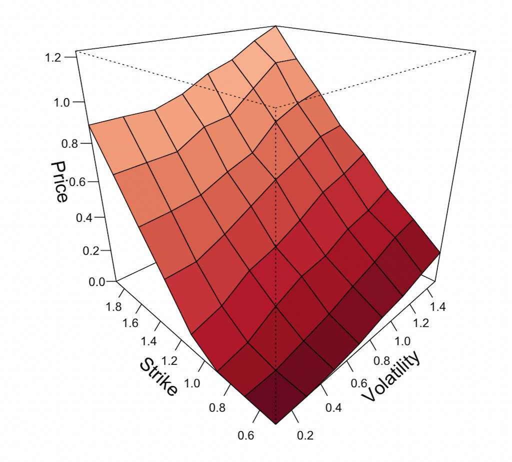By reading the scales of this graph, we can deduce that:

1. Higher volatility enhances an option’s price (more risk, so more premium).

2. Lower volatility diminishes an option’s price (less risk, so less premium).

3. In the case of a put option (as simulated by this software), the value of the option decreases close to or exactly zero as the option ventures further in-the-money (ITM).

4. The more out-of-the-money (OTM) the option is, the higher the value of the option to compensate the investor for the level of risk involved.

#2

This code places more input parameters into the simulation than the first.

put2 <- AmerPutLSMPriceSurf(Spot = 100, vols = (seq(0.1, 2, 0.1)), n = 1000, m = 1,
strikes = (seq(90, 110, 1)), r = 0.06, dr = 0, mT = 1/12)
summary(put2)

In the previous code we simply went with the defaults placed into the program.

Naturally, given that the spot price of the underlying asset is very likely to not be 1.00 (the default), maturity time (mT) may not be 1 (one year), and the current interest rate and dividend rate will be certain values, it can be of strong use to place these directly into the code.

For an option with a month to go until expiry, we can input 1/12 (i.e., one-twelfths of one year).

For an option with two days remaining, 2/365.

Here we labeled the object as “put2” – therefore, if we wanted to derive summary statistics for this function we could simply write “summary(put2)” in order to cull these from the program.

#3

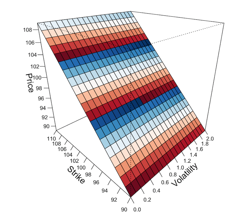
This code uses the Asian American pricing input. We followed the same procedure as used in the previous example.

price_surf<-AsianAmerPutLSMPriceSurf(vols = (seq(0, 2, 0.1)), n=200, mT=1/12,
strikes = (seq(90, 110, 1)))
summary(price_surf)
plot(price_surf, color = divPalette(150, "RdBu"))

We can also produce a graphic of the results:

#4

This code allows you to price American options using the Black-Scholes solution:

#EuPutBS(Spot, sigma(vol), Strike, r, dr, mT) EuPutBS(100, 0.2, 110, 0.06, 0.02, 1/12) EuCallBS(1, 0.2, 1, 0.06, 0, 1)

The option will be evaluated according to its six main valuation criteria:

1. Spot rate (price of the underlying)

2. Sigma (volatility)

3. Strike price (price at which it’s purchased)

4. r (interest rate)

5. dr (dividend rate)

6. mT (maturity time)

#5

Here we can generate options pricing according to standard Brownian motion.

a<-fastGBM(Spot = 1, sigma = 0.2, n = 10000, m = 30, r = 0.06, dr = 0, mT = 1/12)
mean(a)
median(a)
sd(a)
pnorm(1,mean(a),sd(a))

Brownian motion is modeled by the following differential equation nested in the “fastGBM” command:

dS/S = (mu)*t + (sigma)*dWWhere t is time, W is a stochastic variable denoting Brownian motion, and mu and sigma are constants.

In the lines following, one can obtain the mean value produced by the function.

The code will generate 300,000 (n*m) total data points from the above iteration. Naturally the mean it will fall to nearly exactly 1 if r and dr are set to 0.

Adjusting r upwards will cause the value to normally rise above 1. Adjust dr upwards will cause the value to typically go below 1.

One can also calculate standard deviation and, with pnorm(), the percent of the time that price falls below a certain value based on the mean and standard deviation.

To find the percent of time that price falls above a certain value, 1-pnorm(x, mean(a), sd(a)) can be used.

#6

This function evaluates the price of an American put with the Least Squares Monte Carlo method, like in #2.

This code simply shows a different method by which the average price can be extracted from the data points.

put<-AmerPutLSM(Spot = 50, Strike = 45, sigma = 0.2, n = 10000, m = 30, r = 0.06, dr = 0, mT = 1/12)
put$price

#7

This method evaluates the price of an American put option using antithetic variates, which attempts to improve the results by limiting the variance in the simulation.

AmerPutLSM_AV(Spot = 100, sigma = 0.2, n = 1000, m = 365, Strike = 110, r = 0.06,
dr = 0, mT = 1) put <- AmerPutLSM_AV(Spot=50, Strike=52.5, sigma = 0.1, n=200, m=40, r = 0.03 dr = 0.015, mT = 1/4) summary(put) put$price

Two sample codes are provided. The first offers an option with a yearly expiry; the second, a quarterly expiry.

#8

The AmerPutLSM_CV function estimates an option’s price via the Least Squares method using control variates.

It serves as another reduction technique by using the solution to a known quantity to reduce the variance in the unknown. In this case, the Black-Scholes solution for a European put option serves as the control.

AmerPutLSM_CV(Spot = 1, sigma = 0.2, n = 1000, m = 365, Strike = 1.1, r = 0.06,
dr = 0, mT = 1) put <- AmerPutLSM_CV(Spot=142, Strike=165, n=200, m=50) summary(put) put$price

Two example codes are provided.

By using a proxy naming command to denote an object (“put” in the second code above), the summary() function can be used to derive all the input parameters.

#9

The following code allows one to calculate the price of quanto American puts.

A quanto option is an exotic investment instrument by which the payoff is cash-settled, but in the form of a different currency from which was used to instigate the initial trade at a predetermined price or exchange rate.

Quanto options are of interest to speculators and investors who want to invest in a different currency but don’t wish the undertake the associated exchange rate risk due to the stipulated predefined payoff rate.

For instance, if an investor wished to invest in the Euro, he or she could purchase a quanto option in USD at a predefined exchange rate, and upon settlement receive Euros in return.

put <- QuantoAmerPutLSM(Spot=69.33, Strike=73.5, n=5000, m=1, r = 0.04, dr = 0.03, mT = 1/12)
put
summary(put)

Writing the object name “put” will allow you to see example values of the simulation. The summary() command summarizes the option’s price determined by the simulation, plus all relevant input parameters.

#10

Quanto option Monte Carlo simulations can also be determined through antithetic variates.

 put <- QuantoAmerPutLSM_AV(Spot = 10, sigma = 0.10, n = 1000, m = 365, Strike = 11.5, r = 0.05, dr = 0.01, mT = 1, Spot2 = 15, sigma2 = 0.2, r2 = 0, dr2 = 0, rho = 0) summary(put)

In this case, we are introducing the corresponding asset in which the quanto option would be paid via Spot2, sigma2, r2, and dr2.

The rho input denotes the correlation coefficient between the two underlying assets.

This code models the way in which an investor might invest in the $10 (Spot) asset and be paid out in terms of the £15 asset (Spot2), or whatever the designated currency happens to be.

Conclusion

These ten code examples will help you gain familiarity with simulating options prices via the Least Squares Monte Carlo method.

Monte Carlo coding can become convoluted the more extensive the financial model becomes, but having a package such as LSMonteCarlo to work with in R makes the process easier and greatly enhances time efficiency.

Additional Notes

Just a couple quick notes on how interest rates and dividend yields affect an option’s price:

A higher interest rate, r, will lower the price of an option.

This makes borrowing money more expensive, and both businesses and consumers will decrease their spending accordingly.

This is bad for business as a whole and will cause stock prices to fall. The price of the option will lower automatically due to interest rate changes.

A higher dividend rate, dr, will increase the price of an option.

A stock with a higher dividend rate is a more valuable one as investors receive a fraction of the value of their holdings in that stock. The price of the option will increase as a result.

The time until maturity also has an effect. An option with a year-long expiry will naturally be of more value than an option with a month-long expiry.

This is more risk inherent in an option of one year as it gives time for the underlying asset to fluctuate in price.

And with more risk comes a higher value to the option and therefore a higher premium that can be collected by the seller of the option.