Lattice Models in Finance & Trading

Lattice models have widespread use in the valuation of financial derivatives, risk management, and trading/investment strategy development.

They provide a structured, discrete framework for modeling the evolution of financial variables over time.

This makes them most useful in scenarios where continuous models are either too complex or inappropriate.

Key Takeaways – Lattice Models

• Flexibility in Pricing
  • Lattice models, like binomial trees, allow for the pricing of complex options, including for American options which can be exercised anytime.
• Risk Management Tool
  • They enable traders to assess and hedge risks by simulating various market scenarios and option outcomes.
• Applicable Across Assets
  • These models are versatile and useful for equities, interest rates, and credit derivatives.
• Coding Example
  • We do a Python coding example of a lattice model (binomial tree) below.

Here’s an overview of their application in finance, markets, and trading:

Lattice Option Pricing Models

Binomial and Trinomial Trees

These are the most common lattice models used for option pricing.

The binomial model breaks down the time to expiration of an option into potentially a large number of time intervals, or steps.

At each step, the price can move up or down by a specific factor.

Trinomial trees extend this concept by allowing three possible movements: up, down, or unchanged.

We do binomial tree coding examples at the bottom of this article.

Flexibility in Modeling

They’re very useful for American-style options, which can be exercised at any time before expiration, as they can easily accommodate the option’s path-dependent features.

Interest Rate Lattice Models

Modeling Bond Prices and Yields

Lattice models can simulate the evolution of interest rates over time.

This helps in the pricing of interest rate derivatives like bond options and caps and floors.

Hull-White and Black-Derman-Toy Models

These are examples of lattice models applied to interest rate movements.

Lattice Models in Credit Risk Modeling

Default Probability Estimation

They are employed to estimate the probability of default of a bond issuer or counterparty in a derivatives transaction.

Credit Exposure

Useful in calculating potential future exposure of derivative positions.

Takes into account possible defaults.

Lattice Models in Real Options Analysis & Corporate Finance Decisions

Used for analyzing investment decisions in real assets, where the optionality arises from management’s ability to make future decisions that affect the value of the project or investment.

Lattice Models in Portfolio Management & Asset Allocation

Strategic Allocation

Can be used to model the behavior of asset prices under different economic scenarios.

Assists in strategic asset allocation.

Risk Management

Helps in assessing the risk profile of a portfolio under various market conditions.

Lattice Models & Market Simulations

Lattice frameworks can be an alternative to Monte Carlo simulations for modeling the behavior of asset prices, especially when dealing with path-dependent options or complex derivatives.

Math Behind Lattice Models

Here is a brief overview of the math behind lattice models for options pricing:

The basic idea is to discretize the continuous stochastic processes from models like Black-Scholes into a lattice or tree structure (i.e., break it into very small steps).

Some key equations

The asset price at each node follows a binomial distribution*:

S(t+Δt) = S(t)u, with probability p

S(t+Δt) = S(t)d, with probability 1 – p

Where u and d are the up and down factors:

u = e^σ√Δt

d = 1/u

The risk-neutral transition probabilities are:

p = (R – d)/(u – d)

1 – p = (u – R)/(u – d)

Where R is the risk-free rate over the period Δt.

The parameters u, d, and p are calibrated to real world data.

The option price is calculated backward from the final nodes using the risk-neutral valuation:

C(t) = (p*C(t+Δt, up) + (1-p)*C(t+Δt, down))/R

Where C(t) is the option price at time t, and C(t+Δt, up) and C(t+Δt, down) are the option prices at the up and down nodes at t+Δt.

By stepping backward through the tree, the initial option price C(0) can be calculated.

The lattice provides a discrete approximation to the continuous process.

There are different formulas depending on the option type (call/put) and exercise timing (European/American).

*(Note that the assumption of a binomial distribution only holds for the change in the asset price. The actual asset price distribution will not be perfectly binomial.)

Advantages of Lattice Models

Flexibility

They can be adapted to various types of derivatives and underlying assets.

Computational Efficiency

Generally more computationally efficient than continuous models for American-style and exotic options.

Limitations of Lattice Models

Simplicity vs. Reality

The simplistic up/down movement might not capture the real-world complexities of financial markets.

Discretization Errors

As they discretize time and price movements, there can be errors compared to continuous models.

Limited Number of Discrete Paths

Lattice models only follow a certain number of discrete paths.

Alternatives to Lattice Models

Alternatives to lattice models in financial markets include:

Black-Scholes Model

A continuous-time model for pricing European options.

Black-Scholes is a closed-form solution that simplifies calculations but may not accurately handle American options or path-dependent features.

Monte Carlo Simulations

Used for pricing complex derivatives and evaluating risk by simulating thousands of potential future paths for asset prices.

Incorporates a wide range of market conditions.

Finite Difference Methods

Numerical techniques for solving differential equations arising in option pricing.

Useful for a variety of exotic options and capable of handling American-style exercise features.

Local Volatility Models

Extend the Black-Scholes framework by allowing volatility to vary with both time and the underlying asset’s price.

Summary

These methods offer different strengths, from computational efficiency to the ability to model complex market behaviors.

They provide quant traders and financial engineers with a toolkit for various scenarios.

Recent Developments & AI Integration

Integration with Machine Learning

AI and machine learning are being used to enhance lattice models, especially in calibrating model parameters more effectively.

High-Frequency Trading

In algorithmic and high-frequency trading, lattice models might be integrated into strategies for pricing and risk management.

Coding Example – Lattice Models

The binomial tree model is a discrete-time model used for pricing options, and commonly used for American options, which can be exercised at any time before expiration.

The model works by breaking the time to expiration into a number of discrete intervals, or steps.

At each step, the stock price can move up or down by a certain factor, and the option value is calculated backward from expiration to the present.

Below is a simple Python implementation of a binomial tree model for a European call option.

We’ll use a European option for simplicity since its valuation does not require checking for early exercise at each step (unlike an American option).

Nevertheless, the logic is quite similar, and this can easily be extended to American options with minor modifications.

import numpy as np

def binomial_tree_call_option(S0, K, T, r, sigma, N):
    """
    Price a European call option using the binomial tree model.

    Parameters:
    S0 : float
        Initial stock price
    K : float
        Strike price of the option
    T : float
        Time to maturity in years
    r : float
        Risk-free interest rate
    sigma : float
        Volatility of the underlying asset
    N : int
        Number of steps in the binomial tree

    Returns:
    float
        Price of the European call option
    """
    # Calculate delta T
    deltaT = T / N

    # Calculate up and down factors
    u = np.exp(sigma * np.sqrt(deltaT))
    d = 1 / u

    # Calculate risk-neutral probability
    p = (np.exp(r * deltaT) - d) / (u - d)

    # Initialize our array for stock prices
    stock_price = np.zeros((N + 1, N + 1))
    stock_price[0, 0] = S0

    for i in range(1, N + 1):
        stock_price[i, 0] = stock_price[i - 1, 0] * u
        for j in range(1, i + 1):
            stock_price[i, j] = stock_price[i - 1, j - 1] * d

    # Initialize the option value at maturity
    option_value = np.zeros((N + 1, N + 1))
    for j in range(N + 1):
        option_value[N, j] = max(0, stock_price[N, j] - K)

    # Iterate backwards in time to calculate the option price
    for i in range(N - 1, -1, -1):
        for j in range(i + 1):
            option_value[i, j] = (p * option_value[i + 1, j] + (1 - p) * option_value[i + 1, j + 1]) / np.exp(r * deltaT)

    return option_value[0, 0]

# Example parameters
S0 = 100 # Initial stock price
K = 100 # Strike price
T = 1 # Time to maturity in years
r = 0.05 # Risk-free interest rate
sigma = 0.2 # Volatility
N = 50 # Number of steps

# Calculate the call option price
call_price = binomial_tree_call_option(S0, K, T, r, sigma, N)
print(f"The European call option price is: {call_price}")

This script defines a function binomial_tree_call_option to calculate the price of a European call option using the binomial tree model.

You can adjust the parameters (S0, K, T, r, sigma, N) to fit the specific option you’re interested in pricing.

The model starts by constructing a binomial tree for the underlying stock price over N steps until expiration, then calculates the option value at each node starting from expiration and working backwards to the present.

The risk-neutral probability p is used to weight the expected payoffs in the future, discounted back at the risk-free rate r.

Graph of the Binomial Tree Model

Here’s some code we can use to generate a visual of the binomial tree model to simulate the path of a stock price over time.

import matplotlib.pyplot as plt

def plot_binomial_tree(S0, K, T, r, sigma, N):
    """

    Parameters:
    S0 : float
        Initial stock price
    K : float
        Strike price of the option
    T : float
        Time to maturity in years
    r : float
        Risk-free interest rate
    sigma : float
        Volatility of the underlying asset
    N : int
        Number of steps in the binomial tree
    """
    deltaT = T / N
    u = np.exp(sigma * np.sqrt(deltaT))
    d = 1 / u
    p = (np.exp(r * deltaT) - d) / (u - d)

    # Stock price tree
    stock_price = np.zeros((N + 1, N + 1))
    for i in range(N + 1):
        for j in range(i + 1):
            stock_price[i, j] = S0 * (u ** j) * (d ** (i - j))

    # Option value tree
    option_value = np.zeros((N + 1, N + 1))
    for j in range(N + 1):
        option_value[N, j] = max(0, stock_price[N, j] - K)
    for i in range(N - 1, -1, -1):
        for j in range(i + 1):
            option_value[i, j] = (p * option_value[i + 1, j] + (1 - p) * option_value[i + 1, j + 1]) / np.exp(r * deltaT)

    # Plotting
    plt.figure(figsize=(10, 6))
    for i in range(N + 1):
        for j in range(i + 1):
            if i < N:
                plt.plot([i, i + 1], [stock_price[i, j], stock_price[i + 1, j]], color='gray', lw=1)
                plt.plot([i, i + 1], [stock_price[i, j], stock_price[i + 1, j + 1]], color='gray', lw=1)
            plt.scatter(i, stock_price[i, j], color='blue', s=10) # Stock price nodes

    # Highlight option valuation at maturity
    for j in range(N + 1):
        if stock_price[N, j] - K > 0:
            plt.scatter(N, stock_price[N, j], color='red', s=30) # In-the-money nodes at expiration

    plt.title("Binomial Tree Model of Stock Price and Option Valuation at Expiration")
    plt.xlabel("Time Steps")
    plt.ylabel("Stock Price")
    plt.grid(True)
    plt.show()

# Plot the binomial tree with option valuation
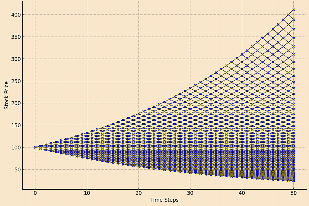
plot_binomial_tree(S0=100, K=100, T=1, r=0.05, sigma=0.2, N=50)

Here is the graph showing the path of the binomial model for the stock price over time, as per the specified parameters.

Each node represents a possible stock price at that point in time.

You can notice the lattice format illustrating how the stock price can evolve through the binomial tree model up to expiration, with a wide distribution of possible outcomes.

This visualization helps in understanding the dynamics of option valuation under the binomial model framework.

Binomial Tree Model of Stock Price

Conclusion

Lattice models remain a fundamental part of financial modeling and analysis.

They offer a blend of theoretical rigor and practical applicability across various domains of finance.

Their adaptability and efficiency make them useful for professionals in financial markets and trading.