Higher-Moment Portfolio Optimization

Modern portfolio theory revolves around creating an optimal portfolio that maximizes the expected return for a given level of risk.

Yet, traditional portfolio optimization methods often consider only the first two moments of the return distribution: mean and variance.

Mean is basically returns – i.e., how much has this asset generated per year or how much is it expected to generate in the future?

Variance is the volatility, typically expressed as a standard deviation. Variance is a type of risk.

This approach overlooks important factors, including skewness and kurtosis, which are key to understanding the return distribution more comprehensively.

So, this article looks at the concept of higher-moment portfolio optimization, demonstrating its significance and application.

Key Takeaways – Higher-Moment Portfolio Optimization

• Traditional portfolio optimization methods, based on Modern Portfolio Theory, focus on mean and variance as measures of expected return and risk, respectively.
• However, these methods overlook skewness and kurtosis, which provide important insights into the distribution of returns.
• Higher-moment portfolio optimization incorporates these skewness and kurtosis measures into the portfolio selection process, allowing for a more comprehensive assessment of risk.
• Skewness measures the asymmetry of the return distribution, while kurtosis quantifies the thickness of the distribution tails.
• By including skewness and kurtosis in portfolio optimization, traders/investors can better manage extreme events and achieve a more balanced portfolio that considers risk and reward in a multidimensional way.
• However, accurate estimation of higher moments can be challenging, and the greater complexity of the optimization process may require advanced computational resources.

Understanding Higher-Moment Portfolio Optimization

Traditional portfolio optimization, rooted in Harry Markowitz’s Modern Portfolio Theory (MPT), incorporates two statistical measures: mean and variance.

The mean represents expected return, while variance signifies risk.

However, only considering these two moments potentially ignores critical information about the investment return distribution.

Higher-moment portfolio optimization introduces the third and fourth statistical moments, skewness, and kurtosis, into the portfolio selection process.

Skewness and kurtosis boil down to this:

• Skewness – asymmetry of the return distribution
• Kurtosis – quantifies the thickness of the distribution tails

Incorporating these additional moments allows for a more comprehensive portfolio risk assessment, accounting for extreme events that could lead to substantial losses (or gains when employed in a favorable way).

Theoretical Framework of Higher-Moment Portfolio Optimization

The objective of higher-moment portfolio optimization is to maximize the expected return of the portfolio, subject to a given level of risk.

This risk is defined not only by variance but also skewness and kurtosis.

The optimization process includes these additional moments into the utility function, leading to a more balanced portfolio that takes into account both risk and reward in a more multidimensional way.

Significance of Skewness and Kurtosis in Portfolio Optimization

In financial markets, returns often exhibit non-normal distributions.

The consideration of skewness and kurtosis provides a more accurate depiction of the return distribution, thus enabling better risk management.

Skewness

Investors generally prefer positive skewness, which represents the potential for large gains and limited losses. (Buying options would be an example of positive skew – assuming the premium isn’t too expensive.)

Negative skewness, on the other hand, implies a risk of severe losses (e.g., selling options).

By incorporating skewness into portfolio optimization, investors can balance their preferences for risk and reward more effectively.

Kurtosis

High kurtosis implies a high probability of extreme returns (either gains or losses), often referred to as “fat tails.”

By considering kurtosis, investors can manage the risk associated with extreme market events that could lead to significant portfolio losses.

In our rundown of various example portfolios, we listed skewness and kurtosis in their summary statistics:

• Harry Browne Permanent Portfolio
• Golden Butterfly Portfolio
• Yale Portfolio (David Swensen Lazy Portfolio)
• Paul Merriman Ultimate Buy & Hold Portfolio
• Gone Fishing Portfolio
• 3-Fund Bogleheads Portfolio
• Scott Burns Couch Potato Portfolio

What creates more favorable skewness and kurtosis?

An easy one is diversifying.

When you diversify in a prudent way, you will achieve more return for each unit of risk.

An example of improved skewness (positive skew) coupled with greater kurtosis is the comparison between the Harry Browne permanent portfolio (linked above) and its comparisons to the 60/40 portfolio and S&P 500.

Another one is being long gamma. This generally means being long options because you have large upside and limited downside.

However, it depends.

It’s important to make sure the options are not too expensive – i.e., when their implied volatility is above their realized volatility.

Practical Implementation of Higher-Moment Portfolio Optimization

Incorporating higher moments into portfolio optimization necessitates more sophisticated mathematical methods, given the added complexity.

Despite the complexity, the development of financial technology and advanced optimization algorithms have made it possible to implement higher-moment portfolio optimization in practice.

This advanced approach requires proper statistical estimation of the return distribution’s moments and correlations.

Moreover, as higher moments are notoriously difficult to estimate with precision, robust estimation techniques are essential to avoid misleading results.

Limitations of Higher-Moment Portfolio Optimization

While higher-moment portfolio optimization provides a more comprehensive risk assessment, it’s not without challenges.

The most significant issue is the accurate estimation of higher moments.

Skewness and kurtosis estimates are often unstable and can lead to misleading outcomes.

Also, including more moments increases the complexity of the optimization process.

The added complexity necessitates more computational power and sophisticated algorithms.

Therefore, higher-moment portfolio optimization may be out of reach for some traders/investors with limited resources.

How Can I Create a Plot of Kurtosis and Skewness for a Particular Portfolio?

You can create a kurtosis and skewness model in any standard statistical computing software.

Below we have an example in R.

We broke it down into five sections, as denoted by the ‘#’ followed by the word description:

install.packages("ggplot2")
install.packages("moments")

library(ggplot2)
library(moments)

# Set parameters
num_simulations <- 1000
num_periods <- 252
returns <- 0.10
volatility <- 0.20

# Generate random returns using Monte Carlo simulation
set.seed(100)
portfolio_returns <- matrix(0, nrow = num_periods, ncol = num_simulations)
for (i in 1:num_simulations) {
portfolio_returns[, i] <- rnorm(num_periods, mean = returns, sd = volatility / sqrt(num_periods))
}

# Calculate skewness and kurtosis for each simulation
skewness_values <- apply(portfolio_returns, 2, skewness)
kurtosis_values <- apply(portfolio_returns, 2, kurtosis)

# Create data frame for plotting
results <- data.frame(Skewness = skewness_values, Kurtosis = kurtosis_values)

# Plotting
ggplot(results, aes(x = Skewness, y = Kurtosis)) +
geom_point(color = "blue", alpha = 0.6) +
labs(x = "Skewness", y = "Kurtosis") +
theme_bw()

In this code, we first set the parameters such as the number of simulations (num_simulations), the number of periods (num_periods), the expected annualized returns (returns), and the volatility (volatility).

We then use a loop to generate random returns for each simulation using the rnorm function.

After that, we calculate the skewness and kurtosis for each simulation using the skewness and kurtosis functions from the moments package.

Finally, we create a data frame with the skewness and kurtosis values and use ggplot2 to create a scatter plot of the results, with skewness on the x-axis and kurtosis on the y-axis.

Make sure you have the ggplot2 and moments packages installed before running this code. (We did this in the first two lines of the code.)

The resulting plot looks like this (and will change slightly, as its based on Monte Carlo simulation):

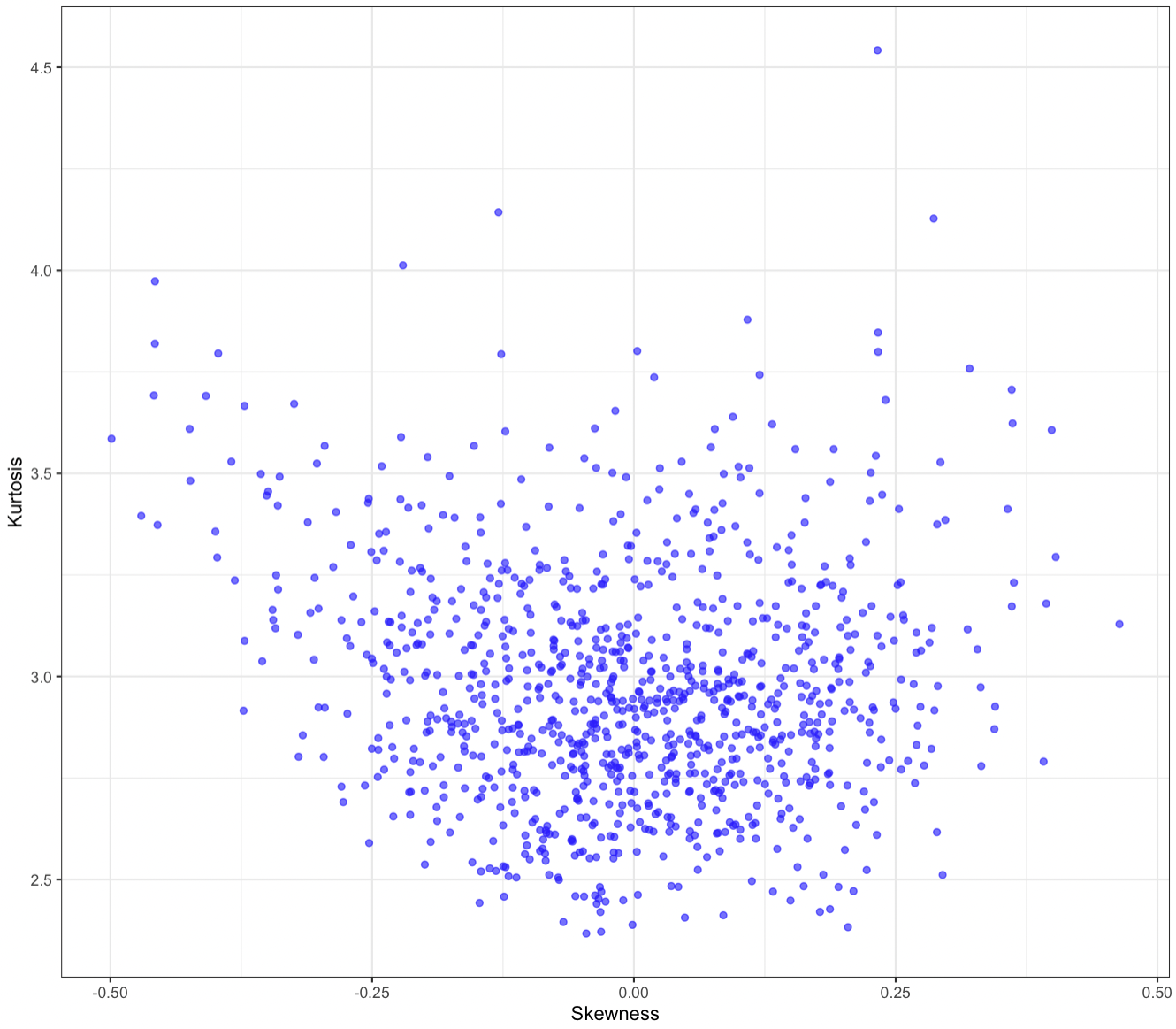
This diagram also illustrates how skewness and kurtosis for a given portfolio are highly variable and not static, especially over short periods of time.

We described more about the basics of Monte Carlo simulation in R in this article.

Conclusion

In financial markets, traditional portfolio optimization strategies may not adequately account for the multifaceted nature of investment risk.

Higher-moment portfolio optimization, which considers skewness and kurtosis, offers a more nuanced and comprehensive view of portfolio risk.