Convexity


Convexity is a concept in finance where there are non-linearities in a potential output after adjusting an input variable.
Namely, in a case where convexity exists, when one variable change, the output changes in a non-linear way.
Mathematically, convexity pertains to the second derivative of the output price with respect to an input price.
In options pricing, this is referred to as gamma (Γ), one of the greeks used in assessing the sensitivity of the price of an option with respect to certain underlying parameters.
The most common use of the term convexity in mathematic finance pertains to bond convexity, which is the second derivative of bond price with respect to interest rates (or yields).
Top Brokers For Trading Convexity
-
1
 Interactive Brokers
 -
2
 NinjaTrader
 -
3
 eToro USAeToro USA LLC and eToro USA Securities Inc.; Investing involves risk, including loss of principal; Not a recommendation
 -
4
 Plus500USTrading in futures and options involves the risk of loss and is not suitable for everyone.
Bond convexity
Bond convexity is an important aspect of bond trading. In basic terms, when interest rates go down, this is good for bond prices. If you own a bond and the interest rate (i.e., yield) on it decreases, that means you’ve made money on it mark-to-market.
But as yields on bonds go down, this also lengthens their duration and makes them more sensitive to changes in interest rates going forward.
Convexity as it pertains to equities
The same is also true for equities. Stocks are another cash flow distribution instrument like bonds. But they tend to be more volatile because the cash flows of equities are theoretically perpetual.
Likewise, when their prices go up, it usually means their forward yields are going down. This lengthens the duration of stocks and similar financial assets. Accordingly, it also makes them more sensitive to changes in interest rates.
When you value a stock based on a required rate of return, notice how the line isn’t perfectly linear.
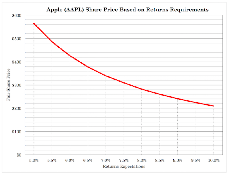
(Source: Apple Stock Trading)
It’s slightly convex or non-linear.
When we valued Apple stock (pre-split) for its fair value at 10 percent required returns, we found its fair value to be at just over $200.
When we valued Apple stock for its fair value at 5 percent required returns, we found its fair value to be at nearly $600.
Even though our returns expectations decreased by a factor of just 0.5x, that didn’t mathematically boost the “fair value” price of the stock by 2x, but by nearly a factor of 3x.
That’s how convexity works in practice.
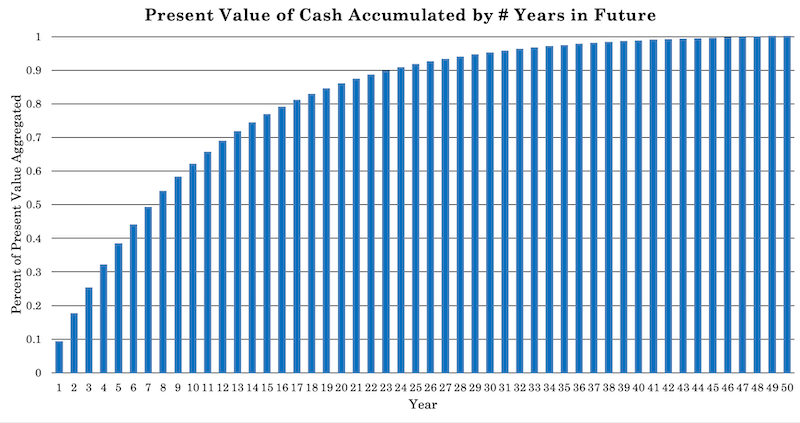
It has to do with the discounting practice. When you invest in a stock, bond, piece of real estate (to rent out), or whatever it is, you put up a lump sum for a future series of cash flows.
A dollar today is worth more than a dollar tomorrow. And this is non-linearly influential.
Under the standard discounting process for a stock (a perpetually cash flow instrument), half of its value might be concentrated in the first seven years or so. While the other half is in the following decades after that.
When a stock is expected to have more of its cash flow in the future because it’s considered a growth stock, it will have longer duration and usually have an even more convex relationship.
Convexity as it pertains to risk management
You can also say portfolio losses follow a convex relationship.
When you lose 10 percent of your portfolio, you need just an 11 percent corresponding return to get back to where you were.
However, if you lose 25 percent, you need a 33 percent gain just to get back.
If you lose 50 percent, then you need a 100 percent return.
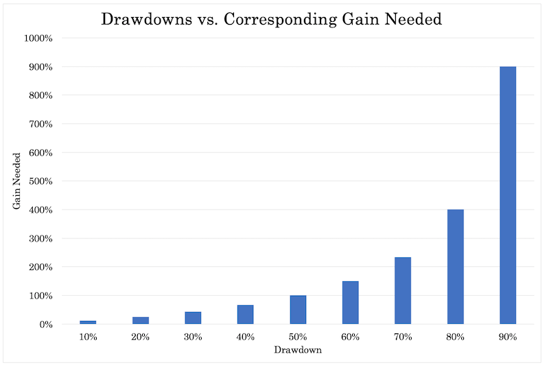
This is why limiting drawdowns is such an important part of trading.
Option convexity
Options are also one of the most common example of convexity in mathematical finance, particularly of the out-of-the-money (OTM) variety.
The further OTM an option is, the greater its convexity.
When one buys an option one is putting up an amount in exchange for the opportunity to potentially own the underlying in the future.
In other words, the downside is capped and the upside can be potentially unlimited. This provides a source of leverage. And once the underlying starts moving in-the-money (ITM) faster than the rate of time decay (theta), the price of the option starts increasing non-linearly.
An easy way to demonstrate this is through a payoff diagram.
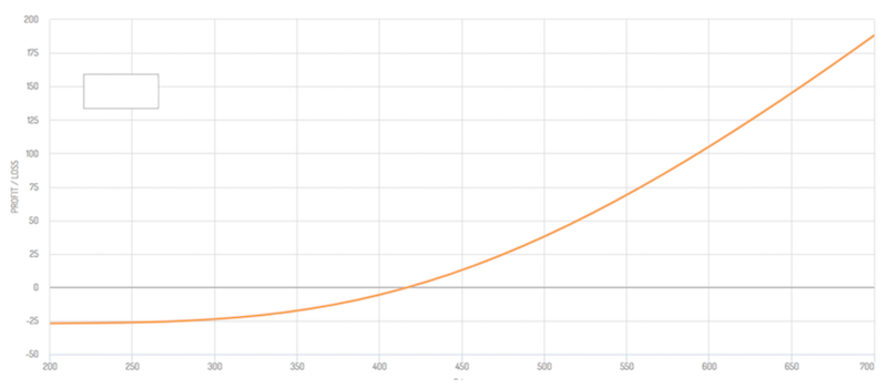
(Source: optioncreator.com)
The value of an option is heavily embedded in the convexity of the potential payout. As the name itself implies, the trader has the option to buy the underlying (in the case of a call option) or sell the underlying (in the case of a put option).
The graph shows a clearly convex payout.
If one buys a call option, then the implication is that the expected value of the payout is higher than the future value of the underlying.
Convexity has much to do with the interpretation of derivative pricing. The price of an option has a lot to do with the embedded optionality – which is reflective of the convexity of the option’s convex payoff function.
You can only lose a small amount, but potentially gain up to many multiples of your premium.
Some traders, as a result of this relationship, believe portfolios should always be long gamma (which means owning options).
Traders who do sell options uncovered will at points learn painfully that you can lose many multiples of your premium.
Owning options is a simple way to cut off left-tail risk completely, limit drawdowns in a certain part of your portfolio, while also keeping the big upside.
That said, selling volatility is certainly viable if done in a smart way.
Many traders also use options not as a means to make bullish or bearish wagers, but for prudent hedging purposes.
Some also sell options as part of a core strategy, by selling options and covering that position by being long or short the underlying (for a call or put option, respectively).
In mathematical terms
Convexity mathematically refers to the second derivative of a modeling function.
With respect to bonds, for example, convexity is the second derivative of price with respect to interest rates. (Duration is the first derivative of price with respect to interest rates.)
In these cases, like with discounted cash flow price outputs while changing the required yield (i.e., rate of return) in the Apple stock price modeling example above, geometrically the price model is not linear but curved.
The higher the degree of this curvature, the higher the convexity.
For a bond investor, for example, let’s say they invest in a particular fixed-income instrument yielding six percent.
Let’s say the bond’s yield goes from 6 percent down to 2 percent. Due to convexity, they will see more price appreciation when the yield of their bond decreases from 4 percent to 2 percent than they would going from 6 percent to 4 percent.
Isolating convexity in practice
A pure convexity bet might best be modeled by buying an at-the-money (ATM) straddle.
A straddle appears as the following:
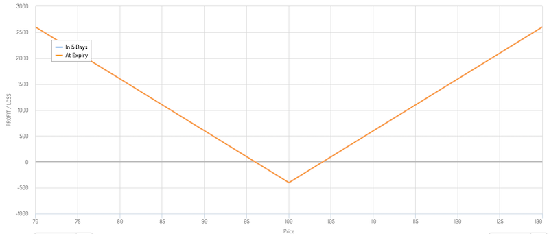
When purchasing at ATM straddle, it is essentially a pure bet on volatility. There is no delta in the trade initially.
Namely, there is no sensitivity to the option value based on the price. One option has a delta of +0.5 (the call) while the other has a delta of -0.5 (the put). The delta nets out to zero.
There is no position taken on the underlying security or instrument. One benefits simply from the extent of movement of the underlying and not the direction.
Delta hedging a convex bet
Some traders will choose to delta hedge a straddle when they do get price movement. This is to essentially take advantage of any volatility they do get.
For example, in the above case, the straddle is bought ATM at $100 per share.
What if the stock goes up to $120 per share over the duration of the trade only to shed all those gains, and finish back at $100 per share by expiration?
The trader would have been right on the movement, having gotten plenty of it, but have nothing to show for it in the end. To avoid this, a trader might delta hedge. We also showed in a separate article how dynamic hedging can help improve return for each unit of risk.
The trade-offs of being long convexity
Like many approaches in trading, there are trade-offs.
Being long convexity – e.g., owning options – also known as being long gamma and often delta-neutral, comes at the trade-off being negative theta.
An option decays over time. One benefits from volatility through the positive gamma position, but loses money over time due to negative theta – also known as theta decay or theta burn.
One will profit if price moves more than expected over the timeframe of the option and lose money on net if price moves less than expected.
Convexity adjustment
A convexity adjustment pertains to the adjustment made to a forward interest rate or yield to obtain the expected future interest rate or yield.
The need for a convexity adjustment has to do with the non-linear relationship between bond prices and their yields. Namely, when a bond yield falls, its price will be higher than what a linear function would assume. (Unless there is negative convexity, which is rare.)
Convexity Adjustment Formula
Convexity adjustment can be broken down into a simple formula:
__
Convexity adjustment = Bond convexity x 100 x (∆r)^2
Where:
∆r = the change in the interest rate or yield
__
Since convexity refers to the non-linear change in the price of a security given a change in the rate of an underlying variable (like a change in yield on bond prices), the price of the output depends on the second derivative of the security’s price with respect to interest rates.
A bond price moves inversely with yields. When interest rates rise, bond prices decline and vice versa.
Therefore, a bond trader knows that interest rates make a big difference on the value of his bond portfolio.
With the changes in the interest rates that occur, the duration of the bond can be calculated.
Duration is the first derivative of a bond’s price with respect to interest rates.
In simple terms, duration is how long it takes a trader or investor to receive his principal back in interest payments (and/or principal).
In slightly more technical terms, duration is the weighted average of the present value of coupon payments plus the repayment of principal.
Duration is measured in years. If a bond’s duration is 10, then it implicitly means that it would take the investor 10 years to receive his principal back in terms of the stream of income received.
It is also a way to estimate the change in a bond’s price for any given change in the interest rate, although it’s not perfect depending on the convexity of the instrument.
For example, if a bond (or financial asset more generally) has a duration of 10, then a one percentage point change in interest rates would change its price by 10 percent.
If interest rates went down by one percent (or 100bps), then the price of the bond would rise by 10 percent.
If interest rates went up by one percent, then the price of the bond would fall by 10 percent.
This is true for all financial assets. It’s true for equities as well.
The price-earnings ratio (P/E) of the stock market is a crude measure of equity duration. If the P/E of the market is 20, that means a one percentage drop in interest rates might expect to generate a 20 percent rise in stock prices.
Convexity, being the first derivative of duration, measures how duration changes along the yield curve. Accordingly, it’s the second derivative for how the price of a bond moves after a change in interest rates.
Because of the convex nature of the yield curve, using the duration estimate for how a change in interest rates would effect prices becomes less accurate the larger the change in yield.
Convexity helps to approximate the change in price that cannot be adequately explained by duration.
A convexity adjustment will look at the curvature inherent in the price-yield relationship displayed in a yield curve to more accurately assess a price change for a prospective change in interest rates.
A convexity adjustment is often necessary for traders to use when pricing bonds, swaps, swaptions, and other types of derivatives because of the asymmetrical change in the price of a financial security in relation to the change in interest rates of yields.
Namely, the percentage increase in the price of a bond for a particular fall in interest rates or yields is always more than the decline in the price for the same increase in rates or yields.
Many factors may influence the convexity of a bond, including its duration, maturity, and coupon payment.
Negative convexity
Negative convexity is rare, but it exists in some circumstances and in some particular corners of the bond market.
When convexity is negative that means the shape of a bond’s yield curve is concave.
For example, most mortgage bonds exhibit negative convexity because of refinancing risk.
When interest rates fall, a homeowner who took out a fixed-rate mortgage will likely try to refinance their mortgage to lock in lower monthly payments.
This is good for the borrower.
But it’s riskier for investors in mortgage-backed securities (MBS) because they are holding onto a bond that’s likely to be paid off faster than what they initially believed.
When interest rates fall, the prices of MBS rise less than other bonds of similar maturities. This is because the amount of time that’s expected to elapse between when the security was issued and when it matures has decreased.
As a result, most mortgage bonds have negative convexity.
Callable bonds
It’s also true for some callable bonds, which normally have negative convexity at lower yields.
With a callable bond, as interest rates fall, the issuer has the increased incentive to call the bond at par. As a result, its price will not rise as quickly as the price of a bond that isn’t callable.
The price of a callable bond might actually drop if the likelihood of the bond being called increases more than the positive influence falling yields have on price. As a result, when yields shrink, callable bonds typically tend to display negative convexity.