Strategies of Derivatives & Volatility Hedge Funds

Derivatives are a way to customize and isolate specific exposures to hedge or create returns streams that are unique from traditional financial assets.

For this reason, they are immensely popular among hedge funds and various institutional investors in terms of how they create value.

Volatility itself is also considered an asset class.

How do these funds generate returns in both calm and turbulent markets and what can you replicate?

We’ll take a look in this article.

Key Takeaways – Strategies of Derivatives & Volatility Hedge Funds

• Derivatives customize risk. You can hedge, leverage, isolate, or customize exposures without owning the asset.
• Volatility is an asset class. Trade the movement itself, not just price direction. Great for hedge funds looking for returns not dependent on traditional asset movements.
• Volatility risk premium exists. Implied vol usually exceeds realized vol over the long-term. This creates carry for sellers. 
  • You can frequently trade this, but it ultimately requires a long-term mindset.
• Two engines of return – long convexity for crashes, short carry for calm regimes.
• Core plays – volatility arbitrage, relative value, dispersion, gamma/vega management, tail hedging.
• Diversify across regimes. Don’t rely on one environment.
• What you can replicate – small, diversified option sells with strict risk limits, occasional long-vol hedges, and disciplined rebalancing.

Understanding Derivatives and Volatility

If you’ve ever watched markets swing up and down and wondered how professionals manage to profit from all that chaos/noise, you’re really asking about derivatives and volatility. 

What Are Derivatives?

At their core, derivatives are financial contracts whose value depends on something else: an underlying asset or exposure. 

That “something else” could be almost anything: a stock, bond, commodity, currency, or even something more complex – e.g., cross-correlations, events, or even another derivative. 

What matters is that a derivative doesn’t have intrinsic value of its own. 

It’s a mirror, reflecting the movements of the underlying market.

There are four main types you’ll hear about: futures, options, forwards, and swaps.

• Futures are standardized contracts traded on exchanges. They obligate the buyer to purchase (and the seller to deliver) an asset at a set price on a future date.
• Forwards are similar to futures, but they’re privately negotiated. More flexible, but also more exposed to counterparty risk.
• Options give you the right, but not the obligation, to buy or sell an asset at a certain price (called the strike). This makes them incredibly useful for managing risk or customizing exposures.
• Swaps are agreements to exchange cash flows, often used to manage interest rate or currency exposure.

The beauty of derivatives is that they let traders shape their exposure in a more precise way. 

You can hedge a position, amplify it, or bet against it entirely, all without ever owning the underlying asset. 

This makes them good for hedging, betting on volatility/prices/certain exposures, and even arbitrage.

Every trader has different goals for why they’re in the trade they’re in. For some, it’s a type of synthetic exposure, some are hedging, and some are betting on volatility, prices, etc.

The Nature of Volatility

Now let’s talk about volatility, or “how much prices move.” 

In financial markets, volatility is a measure of uncertainty or risk (a type of risk, not the sole risk). 

When prices stay steady, volatility is low. When they swing a lot, volatility spikes.

There are two main ways professionals look at volatility:

• Historical volatility measures how much prices have actually moved over time. This gives an idea of what to expect. When they say that US large caps have a “volatility of 15%” it means that historically they’ve moved 15% per year when expressed as a standard deviation. A type of mean expectation.
• Implied volatility looks forward; it’s the market’s dollar-weighted guess about how much prices might move, as inferred from options pricing.

The difference between these two can tell you a lot. 

When implied volatility is high, it means traders expect more price movement ahead (e.g., earnings release, new data, market-wide volatility due to macro shocks, etc.). 

When it’s low, markets are calm, or maybe just complacent or extrapolating recent price action forward.

For hedge funds, volatility is both a risk and an opportunity. 

High volatility can mean sudden losses, but it also opens the door to big returns. 

Many volatility-focused funds actually profit because of volatility; they’re built to profit from it rather than fear it.

In other words, volatility is like wind for a sailor. It can capsize you if you’re unprepared, but if you know how to catch it, it’s what makes the journey possible.

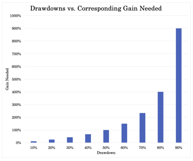
At the same time, there’s also the need to control drawdowns.

You can’t let drawdowns get too far because then it’s very hard to recover from them and the effect is non-linear.

For a 10% drawdown, you need an 11% gain. Almost 1-to-1.

But for a 50% drawdown, you need a 100% gain just to get back.

The Volatility Ecosystem

Over the years, an entire ecosystem has developed around volatility itself. 

There’s even a name for one of its most interesting features: the volatility risk premium. 

This is the consistent tendency for implied volatility (what people expect) to be higher than realized volatility (what actually happens). 

Hedge funds love this gap because from selling volatility (essentially providing insurance) they can collect income over time. And like insurance companies, they can invest the premium income and profit is dependent on premiums and investment income minus what they have to payout.

The main players in this ecosystem include hedge funds, insurers, pension funds, and market makers. 

Each one has a distinct role. 

Insurers and pensions often want to offload risk. 

Hedge funds and market makers, in contrast, are willing to take that risk… if the price is right.

This has led to a surge in volatility-linked products. 

Instruments like VIX futures, variance swaps, and structured notes allow investors to trade volatility directly, rather than just trading the underlying markets. 

Let’s look at the core strategies used by derivative and volatility hedge funds:

Volatility Arbitrage

Volatility arbitrage is about finding moments when the market’s expectations of future volatility don’t match what’s likely to happen. Traders then use that gap, between implied volatility (what the market predicts) and realized volatility (what actually occurs), to generate returns.

You can think of it like betting on the weather. If everyone expects constant storms but you believe the skies will stay calm, you can “sell volatility” and profit when conditions turn out better than forecast. 

Conversely, if you expect rough(er) seas when others expect calm, you “buy volatility.” 

It’s less about predicting direction – it’s generally considered to be market-neutral – and more about predicting the magnitude of movement.

How It Works: The Core Concept

The main idea is to trade the difference between how volatile markets are expected to be and how volatile they actually become.

When implied volatility (from options prices) is low compared to historical volatility, arbitrageurs might buy options, anticipating that future price movements will exceed expectations and hedge out the delta (price movements) to isolate the vega (volatility). 

When implied volatility is high, they might sell options (again, hedging out delta), expecting calmer conditions than discounted. 

The profit comes from the spread between what was priced in and what actually happens.

It’s a strategy built on probabilities and data, not gut feeling. Traders constantly run models to estimate how likely different outcomes are and whether the current pricing of volatility is fair.

The Tools of the Trade

To implement this, hedge funds use a few core instruments:

• Options – The most common vehicle for volatility trades. Buying and selling options lets traders take positions on volatility without betting on direction.
• Volatility Swaps – These allow direct exposure to realized volatility over a set period. They settle in cash based on how volatile the underlying asset actually was.
• Variance Swaps – A more precise cousin of the volatility swap, tied mathematically to the square of volatility. These are often used by institutional traders looking for exact exposures.

Each of these tools gives traders slightly different ways to express the same view, that the market is mispricing uncertainty.

A Simple Example

Imagine the S&P 500’s options market is implying a volatility of 10%, but historically it’s been swinging closer to 15%. (This kind of mismatch tends to occur on shorter horizons, but not always.)

A volatility arbitrageur might buy volatility (for instance, by purchasing options) expecting realized volatility to climb toward that higher level. 

If the market does get choppier and realized volatility rises, those options become more valuable, and the trader profits.

It’s not about predicting where the index will go but about whether it will move more than the market expects.

Example Trade

• Trade = Buy a 1-month at-the-money S&P 500 straddle when implied volatility is 10%. Immediately hedge delta to flat using ES futures. Keep the book delta-neutral by rebalancing as the index moves, so P&L is driven mainly by vega and realized variance.
• Thesis = Realized volatility trends toward 15%, so options reprice higher and the long straddle gains.
• Risks = Theta, slippage, and an implied volatility crush.
• Exit = Close when implied volatility nears 15% or at expiry if realized volatility exceeded carry.

The Hidden Dangers

Of course, volatility arbitrage isn’t risk-free. It’s built on models, and models are only as good as their assumptions. Sudden volatility spikes can blow through even the best-laid plans. Liquidity gaps, times when it’s hard to buy or sell options at fair prices, can also magnify losses.

When markets get stressed, correlations between assets often rise, models break down, and prices move faster than anyone can hedge. What looked like a measured bet on volatility can quickly become a fight for survival.

Relative Value Trading

Relative value trading isn’t about making bold predictions on where markets are headed, but rather about noticing when two related things get out of sync, and betting that they’ll eventually come back together through being both long and short.

Factor investing generally involves relative value, such as “quality minus junk” (QMJ), value (cheap minus expensive), and momentum (long recent winners and short recent losers).

For hedge funds that add value from being uncorrelated from traditional financial assets, relative value is a common strategy.

At its core, relative value trading is about exploiting pricing inefficiencies between related assets or maturities.

Traders might compare two bonds, two stock indices, or two volatility exposures and notice that one looks too cheap or too expensive relative to the other.

Like factors, there may be risk compensation reasons why a relative value trade might work long-term.

The beauty of the strategy is that it’s market-neutral: profits come from relative movements, not the market’s overall direction.

The Core Idea: Finding the Spread

A relative value trader’s job is usually to identify a “spread” – the price difference between two related instruments – and trade it when it deviates from its normal range.

(I usually because some relative value involves a risk premia that endures because of the aforementioned risk premium, such as why cheaper, less volatile companies tend to outperform more expensive, more volatile ones over time.)

Let’s say the spread between two interest rate futures has historically been one point, but now it’s two.

A trader might sell the richer one and buy the cheaper one, expecting the gap to narrow. The trade profits when the relationship returns to equilibrium.

This same idea applies across different asset classes: equities, bonds, credit derivatives, and volatility products.

The key is recognizing relationships that are statistically stable most of the time, and stepping in when they temporarily break.

Common Relative Value Strategies

Calendar Spreads

Calendar spreads involve trading the same asset across different maturities.

For example, a trader might buy a near-term volatility future and sell a longer-term one if the curve looks unusually steep.

The logic is that volatility expectations often revert to normal levels as short-term uncertainty fades.

This approach is especially common in volatility trading, where the term structure (the shape of the volatility curve over time) contains information about discounted expectations.

Let’s look at a payoff diagram of the calendar spread using this trade:

1. Long Option – The trader buys an option with a longer expiration date, usually several months out.
2. Short Option – The trader sells an option with a shorter expiration date, typically the front-month option (that has higher implied volatility).

The horizontal axis of the payoff diagram shows the underlying asset’s price at expiration, while the vertical axis represents the profit or loss of the calendar spread position.

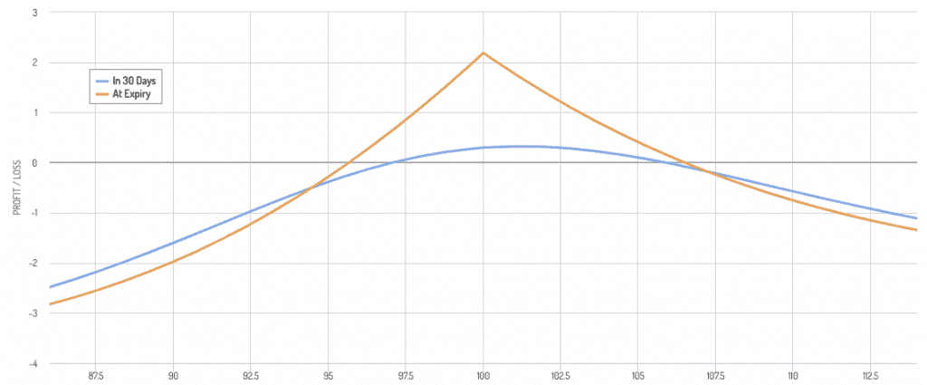
• So, you can see that this is more of a neutral strategy.
• The underlying falling is the worst scenario for the calendar spread.

The payoff diagram assumes that the position is held until expiration.

In practice, traders may choose to exit the position before expiration, depending on what happens and their trading strategy.

Inter-Market Volatility Spreads

Another approach compares volatility levels across related markets; for instance, the S&P 500 versus the Nasdaq.

These indices often move together, but their volatility isn’t always perfectly aligned (the Nasdaq is generally 50-60% higher, on average).

When one index’s implied volatility becomes unusually high relative to the other, traders can buy one and sell the other.

A popular version of this is the long S&P 500 volatility vs. short Nasdaq volatility trade.

The S&P tends to be broader and more stable, while the Nasdaq is more tech-heavy and sensitive to liquidity, interest rates, and growth and inflation expectations.

If tech stocks get overly jittery, the volatility spread between the two indices can widen, which can create an opportunity for mean reversion.

Some will even trade one against the other on a vol-adjusted basis.

For example, if the Nasdaq is, on average, 54% more volatile than the S&P 500, then they’ll short the Nasdaq in a way so that the short is proportionate to the long S&P 500 position (e.g., a 1x long S&P 500 vs. 0.67x short Nasdaq).

The trader would then expect a 1-2% return spread over a full cycle.

Correlation Trades

Correlation trades take this concept one step further by betting on how assets move in relation to each other.

For example, if individual stocks start moving independently while index volatility remains low, a trader might short the index volatility and go long single-stock volatility.

When correlations normalize, the spread converges, generating profit.

Of course, correlations can structurally change as well (e.g., stocks and bonds positively correlating in 2022), so you need to know what you’re doing.

Models and Rebalancing

None of this works without statistical modeling.

Relative value trading relies on analyzing historical relationships and measuring deviations in real time.

For example, traders use regression models, cointegration tests, and AI/ML algorithms to determine when a spread has truly diverged versus when it’s just noise. (Related: Correlation vs. Cointegration)

But identifying the opportunity is only half the battle.

High-frequency rebalancing is critical. Spreads can move fast, and prices can change before trades are fully executed. Automated systems continuously adjust positions, which lock in tiny but consistent profits.

Execution precision, risk management, and transaction cost control often determine success more than the initial insight itself.

Each trade may yield only a small gain, but over hundreds or thousands of trades, those gains compound, especially when the strategy is insulated from broad market swings.

Still, it requires humility. Markets can stay irrational longer than models expect, and spreads can widen before converging.

Tail-Risk and Convexity Strategies

Tail-risk hedging and convexity-based approaches are all about preparing for the kind of market moves traders/investors hope never happen, but inevitably do. 

These tail-risk and convexity strategies help protect portfolios from large, unexpected declines and preserve capital when volatility spikes. 

Whether it’s a rapid 20% loss in a single month or a slow, grinding selloff that lasts a year, the timing and shape of these drawdowns matter a lot.

Both the pace and the path of losses can determine how long it takes to recover and resume compounding returns.

At their core, tail-risk strategies act like financial airbags: they don’t add much value when the road is smooth – they’re more or less a small leak – but when markets crash, they can make the difference between protecting your capital and catastrophe.

As Universa head Mark Spitznagel puts it:

“When the market crashes, I want to make a whole lot, and when the market doesn’t crash, I want to lose a teeny, teeny amount. I want that asymmetry… that convexity.”

Protecting Portfolios from Large, Unexpected Declines

Tail-risk hedging tries to limit large drawdowns in a portfolio, mostly to offset equity declines.

These strategies use derivatives, often options or volatility-linked instruments, to limit downside exposure.

For example, an investor who fears a 25% equity drawdown might buy put options that pay off sharply if the market falls beyond that threshold.

These hedges tend to shine during sudden market shocks like 2008 or 2020, when volatility explodes and correlations among risky assets converge toward one. 

But they’re less effective during slow, grinding declines such as the early 2000s tech bust, which was spread over 3 years (2000, 2001, and 2002 were all red years for US and most global stocks), or the 2022 bond and stock selloff.

In those drawn-out scenarios, options lose value over time, and the protection premium erodes, and the “theta burn” may offset the price falls.

This path dependency, how a drawdown unfolds, matters a lot.

Fast crashes favor option-based hedges because the payoff arrives before time decay sets in.

Prolonged bear markets, on the other hand, slowly eat away at the hedge’s value.

For that reason, professional traders carefully design their protection mix based on whether they fear a quick collapse or a long stagnation.

Long Volatility as Insurance Against Systemic Risk

One of the most direct ways to protect against large losses is by holding long-volatility positions.

These positions increase in value when market volatility rises, often providing a cushion just when traditional assets are falling.

In practice, long-volatility exposure can come from buying put options or owning volatility futures (like VIX futures).

This approach is the financial equivalent of buying insurance. It costs money in good times but pays off well in crises.

That said, long-volatility strategies usually have negative expected returns during calm periods.

Just as you wouldn’t expect to profit from paying car insurance premiums, these strategies erode performance when markets are stable.

Yet when volatility surges, they can offset massive losses elsewhere in the portfolio, preserving both capital and investor confidence.

The Role of Convexity in Asymmetric Payoffs

Convexity is the mathematical backbone of tail-risk protection.

A convex strategy is one where small market moves cost little, but large moves deliver large gains.

Options are a classic example: their losses are limited to the premium paid, while their upside in extreme scenarios can be exponential.

It doesn’t even need to land in-the-money (unless you’re holding to expiration). You just need to get it riding in that direction, with high momentum being the best scenario.

Convexity means that even a small allocation to protection can have a large impact when it’s needed most.

For example, if you allocate 1-2% of your portfolio exposure to deep out-of-the-money puts, for instance, you can transform a devastating 30% loss into a more manageable 10-15% decline.

Of course, the costs can add up, so it’s important to do it judiciously so it isn’t a long-term drag.

This asymmetry, the ability to cap losses while allowing upside, makes convexity strategies attractive for institutions managing long-term capital who needs to cap drawdowns strictly and for some individual investors based on their preferences/needs.

Managing Costs: Balancing Premium Decay with Protection Value

The challenge, as mentioned, is in balancing cost and protection.

Buying protection repeatedly can become expensive due to premium decay, the gradual erosion of an option’s time value.

Over long horizons, this drag can weigh heavily on portfolio returns and impact compounding, especially if crises are infrequent.

Another case is when drawdowns happen, but recovery happens during the options’ life where you ultimately don’t need it.

There are several approaches to managing costs:

• Dynamic hedging – Adjusting hedge levels as volatility changes, reducing exposure when protection becomes too expensive.
• Spreading and structuring – Using combinations of options (e.g., collars, put spreads) to reduce net premiums paid while keeping meaningful downside insurance. You can trade off upside for downside protection.
• Diversifying across strategies – Combining long-volatility, defensive equities, bonds, gold, nominal/inflation-linked bonds, and alternative risk premia to spread out protection sources.

In short, the goal is to own protection that’s cheap enough to maintain yet is strong enough to matter when you need it.

Define what’s not acceptable and hedge against that or figure out ways to reduce the possibility (e.g., diversifying).

Dispersion Trading

Dispersion trading starts with a simple idea. An index is just a bundle of stocks. The volatility of that bundle isn’t the same as the aggregate volatility of the stocks inside it if taken collectively.

To make things more concrete, let’s say the S&P 500 volatility is 15% annualized on average. Yet the volatility of the average single stock in the S&P 500 is around 25%, quite a bit higher than the index.

Dispersion traders try to profit from that gap between index volatility and single-stock volatility.

Trading the Volatility of an Index Versus Its Components

Instead of betting on price direction, dispersion focuses on volatility.

Traders compare implied volatility on an index with implied volatility across its constituents.

If the market is pricing the index as too volatile relative to the names inside it, a trader can take advantage of that.

The trade is market-neutral in spirit.

Example: Short Index Volatility and Long Single-Stock Volatility

A classic expression looks like this:

• buy S&P 500 index options to be long cheaper index volatility, and
• sell a basket of options on the largest single S&P names to be short more expensive single-stock volatility

On the latter, this doesn’t have to be the full index since it’s hard to do 500 positions, but enough so you’re correlated enough.

The index long options give cheaper exposure. The short single-stock options short what’s more expensive, taking advantage of the differential.

If individual stocks bounce around independently while the index stays contained, you can benefit from the convergence.

You still have to manage the Greeks carefully.

Keep deltas near zero, watch gamma and vega, and watch the weights so single-stock exposures map cleanly to index notional.

Your main risks are liquidity and assignment, as well as differences between the index and single stocks.

Gamma and Vega Trading

Active management of option sensitivities (the “Greeks”)

Gamma and vega trading is the art of steering an options book through changing markets by managing its Greeks in real time.

Delta measures directional exposure, gamma measures how fast delta changes, vega measures sensitivity to implied volatility.

Call Gamma (blue) vs. Delta (red)

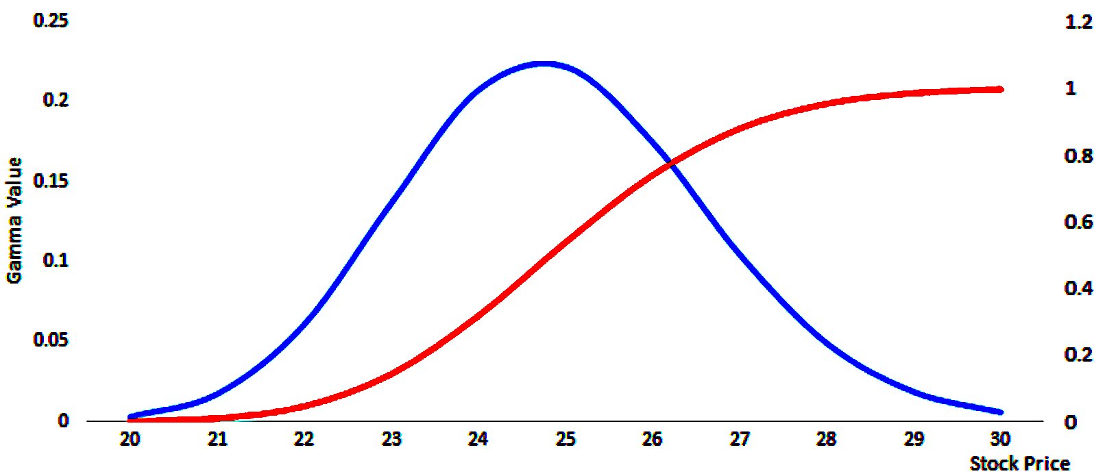
Traders adjust strikes, maturities, and sizes so the book behaves the way they want across small and large moves.

The routine is simple in principle and hard in practice. Keep deltas near target, usually close to flat.

Keep gamma where it matches your plan for intraday swings.

Hold the right vega mix across terms so the portfolio is resilient if volatility shifts. Most of the edge comes from rebalancing and clean execution.

This can be hard for individual traders because of the need to watch Greeks and execute cleanly following predefined rules.

Gamma scalping for income generation

With a long gamma position, your delta rises on rallies and falls on selloffs. If you hedge that delta frequently, you can harvest small gains as prices oscillate.

Buy low when your options make you short, sell high when they make you long. That is gamma scalping.

It works best when realized volatility exceeds what you paid for the options, and when trading costs and slippage are contained.

Positioning also matters. Front-month options carry more gamma per dollar (hence why they’re popular for “gamma squeezes“), but they decay faster.

Further maturities give you a smoother ride, with less scalping income but more staying power if the move stretches out.

Vega positioning to benefit from volatility regime shifts

Vega is your lever for regime change.

If you expect implied volatility to rise, you want positive vega, often through longer-dated options, calendars, or variance exposures that benefit when the whole surface lifts.

If you expect vol to compress, you tilt to negative vega, usually by selling options where supply and demand look favorable, and hedging the tails.

Term structure and skew matter. A steep curve can favor owning near vol against selling far vol, or the reverse, depending on catalysts like central bank meetings, earnings releases, or macro data.

The aim is simple:

• Align vega with the next volatility regime
• keep gamma where you can manage it, and
• let careful hedging turn uncertainty (i.e., implied vol) into a repeatable source of return

Statistical Arbitrage & Quantitative Volatility Models

Individual traders can certainly pursue derivatives and volatility trading and carve out their own success in a way that fits their goals.

But at an institutional level, it’s very math-heavy.

Using quantitative models to forecast volatility dynamics

Quant volatility starts with a simple goal: estimate how much markets will move and when.

Models digest returns, option surfaces, and cross-asset signals to forecast the path of realized and implied volatility.

Classic models include GARCH-type processes (used in markets since the 1980s), state-space models, and regime switches that capture calm versus turbulent periods.

Machine learning and statistical inference in volatility prediction

Machine learning has gone beyond parametrized models. Gradient boosting, random forests, and recurrent networks can learn non-linear patterns that simple models miss.

The job is to predict distributional features, not just a point estimate. That means modeling tails, skew, and jumps.

Cross-validation and walk-forward testing keep you honest. Feature sets mix price dynamics, option-implied measures, macro releases, and microstructure data like order-book imbalance.

Interpretability matters. Use Shapley values or partial dependence to see why the model moves, then pressure test those drivers.

Blending technical and fundamental volatility signals

The best books blend signals so they’re not overly dependent. Technical inputs include, e.g., momentum in vol, term structure slopes, skew shifts, dispersion, correlation.

Fundamental inputs anchor the story: policy paths, earnings cycles, liquidity conditions, and funding stress.

When technicals say vol should fall but policy risk rises, carry trades get smaller and hedges get cheaper.

Positioning follows the signal mix. Own vega when regimes look fragile.

Sell it (carefully) when carry is rich and catalysts are light. Constantly measure realized versus forecast.

Overall, the goal is repeatability.

An individual trader can look at simple cases – e.g., S&P 500 volatility is implied at 30%, which is too high historically and can be profitably harvested if done skillfully – but these are more tactical trades because they don’t repeat very often.

Portfolio Construction and Risk Management

Leverage and Margin Management

Derivatives let you control large exposures with a small capital outlay.

Of course, there are exceptions largely tied to risk/vol expectations. Crypto derivatives require more margin than equity derivatives, which generally require more margin than fixed income derivatives, which require more than rate derivatives.

And in-the-money options (e.g., ITM calls on stocks) are going to require more margin than OTM.

Options, futures, and swaps embed financing in the contract, so you post margin instead of paying full notional.

That frees capital for other ideas and lets you shape risk precisely. The tradeoff is that small market moves can create large P&L swings relative to equity.

The leverage in volatility funds cuts both ways.

Long options cap losses at the premium, yet time decay can grind returns in quiet markets.

Short options harvest relatively steady income (depends on implied vol), yet rare shocks can overwhelm months of gains.

Position limits and pre-set loss thresholds keep this tension in check.

Margin and liquidity are important to track. Funds model initial and variation margin under stress, track collateral needs by counterparty, and pre-arrange funding lines.

Liquidity management links position size to the broader portfolio and everything the market can throw at it.

Stress tests simulate jumps in implied volatility, correlation spikes, and gaps in futures basis. If the book can’t survive a bad tape with widening spreads and slower fills, it’s too big.

Diversification Across Volatility Regimes

Good portfolios don’t depend on up markets when vol is contained or any single environment.

That means combining carry and long-volatility so one pays when the other doesn’t.

Structural hedges sit in the background to protect capital in tail events. You might do these on a one-year horizon (for position traders or investors) so your downside is capped. Tactical trades lean into near-term edges when pricing is off or catalysts are clear.

Building across regimes starts with clear roles. A structural hedge might be deep out-of-the-money equity puts or long variance in a defensive size.

Tactical/alpha overlays can be dispersion, calendar spreads, or correlation relative value.

Scenario analysis brings this to life. You test the book against calm drift, choppy mean reversion, risk-on rallies, and full risk-off.

Backtests help, but they’re only a map. Judgment adjusts for today’s liquidity, positioning, and policy backdrop.

Dynamic Hedging and Position Adjustments

Active management turns static exposures into adaptive ones.

Delta and gamma hedging keep direction risk near target while leaving convexity where you want it.

In a choppy tape, long gamma with frequent hedges can turn noise into income. In a trend, hedging slows and the focus shifts to vega and skew.

Rolling matters. Options decay, term structure shifts, and strikes lose relevance as prices move. Rolling keeps exposure where the risk is.

It also resets collateral and cleans up stale Greeks.

Cross-asset hedging widens the safety net. For example, equity selloffs travel into credit spreads and rates volatility.

A portfolio that can buy credit volatility or own rates convexity alongside equity vega can ride storms with fewer surprises. 

Performance Drivers and Economic Logic

The Volatility Risk Premium

Implied volatility usually sits above realized volatility over time. Investors like insurance and are willing to pay for it.

Market makers demand a margin for warehousing risk. This wedge is the volatility risk premium (VRP).

We can see this, for example, in how Apple’s options traded over the course of one year. The difference between the red line and the zero level is the VRP.

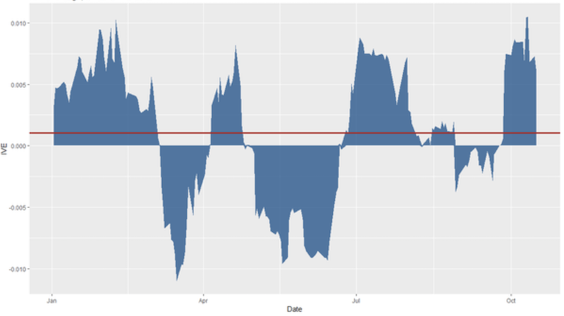
Selling options can turn that wedge into a steady income stream if realized volatility stays tame and your trading/hedging is clean.

As we’ve covered in this article, naturally doing so requires a certain level of sophistication. VRP harvesting isn’t a day trade.

You’ll need to: 

• systematically sell options (e.g., short index puts/calls or put spreads) at prudent sizes, 
• delta-hedge and diversify across maturities and underlyings, and 
• use strict risk limits or tail hedges so that the implied-over-realized volatility wedge accrues as carry. 

It also requires a longer-term mindset. RV will be above IV for periods that will cause those with shorter-term mindsets or those who overleverage to lose confidence.

Premiums aren’t free. In stress, the relationship can flip. Implied volatility can jump too late and then understate the next wave.

Correlation spikes lift index vol more than single-name vol.

Funds/traders that live on selling premium need rules for reducing exposure when risk breaks higher and for re-engaging when panic overshoots fair value.

By and large, the best time to sell premium is when IV spikes in a way that isn’t likely to persist long term.

Even then, remember that everything is probabilistic and even higher probability trades can lose terribly.

Sources of Alpha in Volatility Strategies

Alpha comes from finding edges that persist. Statistical arbitrage – a tech- and expertise-heavy strategy – exploits micro mispricings in surfaces, skews, and term structures.

Behavioral inefficiencies show up when investors overpay for near-term protection or underprice long-dated uncertainty.

Cross-asset signals help time regime change. Rising rates volatility can precede equity volatility. FX volatility can foreshadow credit stress.

Blending these inputs creates a mosaic of signals. No single signal carries the day.

Risk Management and Drawdown Control

Position sizing is the first layer. It keeps losses small and survivable. Tail protection sits at the portfolio level, not just on single trades.

Long volatility in small size can offset correlation breakdowns when everything moves together. Monitoring higher moments matters.

Skew and kurtosis reveal where the book is fragile. The easiest way to improve these metrics is by diversifying.

Benchmarking and Measuring Performance

Vanilla benchmarks include VIX levels, VIX futures curves, and the HFRX Volatility Index.

Many managers add custom indices that match their mix of vega, gamma, and correlation exposure. Returns alone aren’t enough.

Use Sharpe and Sortino to separate signal from noise, then look at skew-aware metrics that account for fat tails.

The most telling statistic is often max drawdown and time to recovery. A smoother equity curve is also especially important to institutional investors.

Fund Examples

Volatility Hedge Fund Archetypes

Volatility sellers’ primary goal is steady income by harvesting the premium between implied and realized volatility.

They focus on diversification, tight risk limits, and disciplined cut points. Their danger is the rare but violent shock.

Volatility buyers pay carry in calm markets to earn in crises. Long convexity is a drag most days, then a lifesaver when everything breaks.

They protect client capital and provide liquidity when others can’t.

Hybrid managers do both. They run core carry with embedded hedges, or they rotate exposure based on regime signals.

The craft is balancing cost and protection so the portfolio compounds.

Integration with Broader Portfolios

Volatility strategies complement stocks and bonds by adding convexity and alternative uncorrelated sources of return.

In multi-strategy funds, they act as both ballast and opportunistic alpha. Institutions use derivatives to trim drawdowns, smooth funding ratios, and match liabilities.

A small sleeve of long volatility or dispersion can reduce the need to de-risk at the bottom. Ideally you want to be buying during such drawdowns.

Derivatives also improve returns through overlays that free up cash while keeping exposure.

Historical Context

In 2008, long volatility and tail hedges paid when correlations converged, as is standard in the tails. Dispersion struggled, then recovered as cross sections reopened.

In March 2020, the fastest drawdown since the Great Depression, punished short volatility and rewarded convexity again.

Post-2022, inflation and rates volatility reshaped many market assumptions – most notably the stocks-bonds correlation, which had previously been thought to diversify each other. Strategies that linked equity, rates, and credit volatility adapted faster.

Structural and Operational Challenges

Model Risk and Assumptions

Quantitative models simplify a messy world. They don’t capture every jump, crowding risk, or policy shock.

Fat tails and volatility clustering break normality (“bell curve”) assumptions.

Stress tests push parameters to extremes and ask what happens if correlations jump, GDP falls 20%, inflation goes to 50% annualized, liquidity halves, and volatility of volatility doubles.

Yes, some of those sound absurd, but no matter what your portfolio throws at you in life, will it go through it without breaking?

Execution and Transaction Costs

Slippage and market impact mean that some edges aren’t actually possible.

Execution algorithms route intelligently, pause in thin books, and avoid predictable footprints around auctions and prints.

They try to avoid giving off information in their order patterns.

The Path Forward for Derivative and Volatility Strategies

The Impact of Technology

AI and ML are changing how things are done. Non-linear models parse option surfaces and order-flow signatures.

Dashboards flag crowding, basis dislocations, and stress in real time. The human edge is shifting more toward framing questions, validating signals, and deciding when to trust or override the machines.

Expanding Volatility Beyond Equities

Volatility alpha is no longer an equity-only game.

Rates, credit, commodities, and FX offer rich term structures and cross-asset links.

Macro and volatility trading are converging. Many macro funds trade vol. A rates shock can drive equity index vol more than an earnings season.

Funds that connect these dots will find edges where single-asset silos can’t.

Evolving Investor Demand

Institutions are adopting volatility overlays and tail-risk sleeves to better stabilize funded status and reduce any chances of forced selling in drawdowns.

That said, the further we get from years like 2020 or 2008 the less important it seems because those bad memories fade.

There’s a steady shift toward systematic and factor-driven volatility funds that offer transparency and capacity.

Clients want fewer surprises and better conversation around costs, convexity, and expected behavior across regimes.

Conclusion

Derivatives give modern hedge funds a precise way to shape risk and return.

Volatility is both the hazard to manage and the raw material to harvest, which is what makes trading volatility unique.

The funds that thrive balance leverage with liquidity, carry (which tends to be anti-convex) with convexity, and quant models with traditional human judgment. 

Over full cycles, success belongs to the managers who protect the downside, respect the math, and keep their compounding alive when others can’t.