Asset Cointegration


Related securities and assets – most stocks, oil and natural gas – often move together in the market over long periods of time.
This reflects a financial concept known as cointegration.
Cointegration occurs when asset prices move together over the long term, even if they may diverge in the short term.
While correlation is by far the more popular concept in finance, cointegration focuses on long-term equilibriums.
Understanding this concept is important for traders and investors, as it forms the basis of strategies like pairs trading, diversification (owning non-correlated/non-cointegrated assets), and can be important for effective portfolio risk management.
Owning assets that have different environmental biases is one of the keys to having a well-diversified portfolio.
Key Takeaways – Asset Cointegration
- Long-Term Relationship
- Cointegration identifies a long-term equilibrium between asset prices, such as stocks and commodities – indicating they move together over time even if they diverge short-term.
- Strategic Importance
- Understanding cointegration is important for trading strategies like pairs trading.
- Also helps understand whether a different asset brings diversification value to a portfolio.
- Just because two assets are cointegrated doesn’t mean they can’t have diversification potential.
- Check correlations, too. (Negative correlations can also indicate cointegration.)
- Dynamic
- Cointegration relationships can change.
- Traders need to continually analyze these relationships and understand the economic forces behind them to make good decisions.
What is Cointegration?
Cointegration represents a statistical phenomenon where two or more time series, like asset prices, move together over the long haul.
Cointegration implies a stable equilibrium relationship despite short-term deviations.
This enduring connection means that, although the assets’ prices may deviate temporarily, they share a common stochastic trend and will revert to an equilibrium relationship over time.
Economic Basis of Cointegration
The existence of cointegration between assets often stems from economic linkages, market forces, or arbitrage opportunities that maintain the long-term equilibrium.
Can Cointegration Mean a Negative Long-run Price Relationship?
Yes, cointegration can represent a negative long-run relationship between the prices of two assets or variables.
Cointegration indicates that two non-stationary time series move together in the long run – i.e., returning to an equilibrium relationship after short-term deviations.
But this long-run equilibrium relationship doesn’t have to be positive.
The cointegrating coefficient, which measures the long-run relationship between the variables, can take on positive or negative values.
A negative cointegrating coefficient implies that the two variables have an inverse or “negative” long-run relationship.
For example, if we look at the prices of a substitute good (e.g. soybean oil) and a competing good (e.g. vegetable oil), we may find that they are cointegrated with a negative coefficient.
This means that in the long-run, when the price of one good increases, the price of the other tends to decrease as consumers substitute toward the relatively cheaper good.
So in essence, while cointegration indicates co-movement and a tendency to not drift too far apart over time, the direction of that long-run relationship (positive or negative) isn’t known from cointegration alone.
A negative correlation coefficient can represent an inverse long-run price relationship between the cointegrated variables.
Example
We can see cointegration if we take perfect negative correlation assets (NASDAQ ETF and short NASDAQ ETF):
| Dependent | Independent | Test Statistic | p-value | 95% Confidence | 90% Confidence |
|---|---|---|---|---|---|
| ProShares UltraPro Short QQQ (SQQQ) | Invesco QQQ Trust (QQQ) | -6.440 | 0.01 | Cointegrated | Cointegrated |
Cointegration Examples
GOOG & SPY
Let’s take the example of Google (GOOG) and the S&P 500 ETF.
We would expect these two assets to be cointegrated – a big component of the index within that index.
We find they’re cointegrated at a 97% confidence interval.
| Dependent | Independent | Test Statistic | p-value | 95% Confidence | 90% Confidence |
|---|---|---|---|---|---|
| SPDR S&P 500 ETF Trust (SPY) | Alphabet Inc Class C (GOOG) | -2.148 | 0.03 | Cointegrated | Cointegrated |
Gold Miners (GDX) & Gold (GLD)
We might expect gold miners (GDX) and gold (GLD) to be cointegrated because the value of gold is naturally a big driver of the value of gold mining companies.
But they also have separate influences as well.
Gold miners and gold being cointegrated at the 90th confidence interval but not at the 95th confidence interval suggests that while there’s a long-term relationship between the two assets, the relationship is not as strong or reliable as it would be if they were cointegrated at the higher 95th confidence level.
| Dependent | Independent | Test Statistic | p-value | 95% Confidence | 90% Confidence |
|---|---|---|---|---|---|
| VanEck Gold Miners ETF (GDX) | SPDR Gold Shares (GLD) | -1.669 | 0.09 | Not cointegrated | Cointegrated |
This suggests there’s a lot of overlap in the buying and selling of gold miners and gold, but some differences as well – some traders/investors would prefer to just own gold while others would prefer to have exposure to gold miners as a business but not the commodity itself.
Nominal Treasury Bonds (TLT) & Inflation-Linked Treasury Bonds (TIP)
Nominal Treasury bonds (TLT) and inflation-linked Treasury bonds (TIP) being cointegrated at the 90th confidence interval but not at the 95th confidence level suggests that there’s a long-term relationship between the two assets, but it’s not as strong or reliable as it would be at the higher 95th confidence level.
This is because while both are Treasury bonds, nominal bonds don’t account for inflation, whereas inflation-linked bonds are designed to adjust their principal and overall payout to account for changes in inflation rates.
This creates a divergence in their behavior in some environments.
| Dependent | Independent | Test Statistic | p-value | 95% Confidence | 90% Confidence |
|---|---|---|---|---|---|
| iShares 20+ Year Treasury Bond ETF (TLT) | iShares TIPS Bond ETF (TIP) | -1.686 | 0.09 | Not cointegrated | Cointegrated |
SPY-GLD
As you get to more fundamentally different assets like stocks (SPY) and gold (GLD) or bonds (TLT) and commodities (GSG), you would expect them to not be cointegrated at a very high confidence interval.
We see a p-value of just 0.35 for SPY-GLD, suggesting there’s a high chance that they’re not cointegrated.
| Dependent | Independent | Test Statistic | p-value | 95% Confidence | 90% Confidence |
|---|---|---|---|---|---|
| SPDR Gold Shares (GLD) | SPDR S&P 500 ETF Trust (SPY) | -0.848 | 0.35 | Not cointegrated | Not cointegrated |
Like with everything, they might have short-term correlations.
TLT-GSG
For bonds and commodities we see a p-value of 0.03.
| Dependent | Independent | Test Statistic | p-value | 95% Confidence | 90% Confidence |
|---|---|---|---|---|---|
| iShares S&P GSCI Commodity-Indexed Trust (GSG) | iShares 20+ Year Treasury Bond ETF (TLT) | -2.124 | 0.03 | Cointegrated | Cointegrated |
So, equities and commodities are cointegrated.
But don’t they bring unique exposures to the portfolio?
Let’s look deeper into this…
Can Assets Be Uncorrelated But Cointegrated (and Vice Versa)?
Yes, assets can be uncorrelated but still be cointegrated.
Cointegration and correlation are two different statistical concepts.
- Correlation measures the degree to which two variables move together in the short-run.
- Uncorrelated assets have no linear relationship in their short-term price movements.
- Cointegration looks at the long-run relationship between variables.
- Two assets are cointegrated if they share a common stochastic drift, meaning their prices may diverge in the short-run, but they tend to move together over the long haul, never drifting too far apart.
So while asset prices may be uncorrelated (no linear short-term relationship), they can still be cointegrated if there is a long-run economic force, like an equilibrium relationship, that links their prices together over time.
Their short-term uncorrelated movements are considered temporary deviations from this long-run equilibrium relationship.
In short, lack of short-term correlation doesn’t preclude the existence of cointegration and a long-run equilibrium tendency between assets.
Uncorrelated but cointegrated assets can occur, especially in financial markets.
Related: Correlation vs. Cointegration
Identifying Cointegrated Assets
Detecting cointegration involves statistical tests like the Engle-Granger or Johansen tests, which help to understand whether assets move together in the long run.
Testing Methods
These tests are designed to uncover whether a long-term equilibrium relationship exists.
Software Tools
Analytical software in Python or R can be used to conduct these tests, which can help in identifying cointegrated pairs or groups of assets.
Caveats
These tests suggest the presence of cointegration, but they don’t confirm it definitively.
Traders/investors must consider the possibility of changing relationships over time.
Python Code for Cointegration Test
Using Synthetic Data
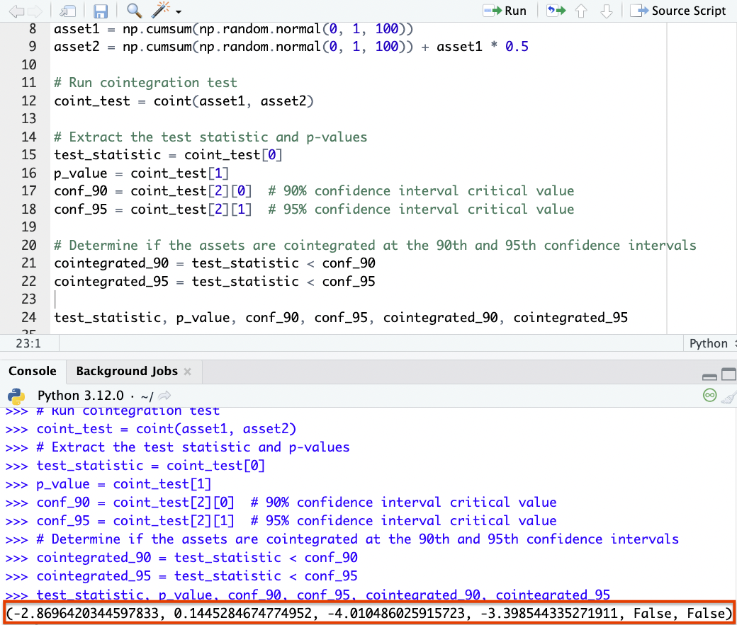
Here’s some Python code you could run for a cointegration test:
import numpy as np
import pandas as pd
import statsmodels.api as sm
from statsmodels.tsa.stattools import coint

# Generate synthetic data for 2 assets
np.random.seed(11)
asset1 = np.cumsum(np.random.normal(0, 1, 100))
asset2 = np.cumsum(np.random.normal(0, 1, 100)) + asset1 * 0.5

# Run cointegration test
coint_test = coint(asset1, asset2)

# Extract test statistic & p-values
test_statistic = coint_test[0]
p_value = coint_test[1]
conf_90 = coint_test[2][0] # 90% confidence interval critical value
conf_95 = coint_test[2][1] # 95% confidence interval critical value

# Determine if the assets are cointegrated at the 90th & 95th confidence intervals
cointegrated_90 = test_statistic < conf_90
cointegrated_95 = test_statistic < conf_95

test_statistic, p_value, conf_90, conf_95, cointegrated_90, cointegrated_95
We can see within this particular example that it’ll say “(False, False)” if the assets are not cointegrated at either the 90th or 95th confidence interval.
Using Real Data
To analyze real data for cointegration between two assets using price data from a CSV file, you can structure your Python code as follows:
Import Libraries
- Import necessary Python libraries for data manipulation and statistical analysis.
Load Data
- Load the price data of the two assets from a CSV file using pandas.
Data Preprocessing
- Make sure the data is clean and aligned by date, handling any missing values if necessary.
Run Cointegration Test
- Use the coint function from statsmodels to test for cointegration between the two price series.
Interpret Results
- Check the test statistic against the critical values to determine if the assets are cointegrated.
Here’s how you can structure the code:
import pandas as pd
import statsmodels.api as sm
from statsmodels.tsa.stattools import coint

# Load data from CSV
def load_data(file_name):
    return pd.read_csv(file_name, index_col='Date', parse_dates=True)

# Main function to test cointegration
def test_cointegration(asset1_data, asset2_data):
    coint_test = coint(asset1_data, asset2_data)
    test_statistic, p_value, critical_values = coint_test
    cointegrated_90 = test_statistic < critical_values[0] # 90% confidence
    cointegrated_95 = test_statistic < critical_values[1] # 95% confidence

    return {
        'test_statistic': test_statistic,
        'p_value': p_value,
        '90%_conf': cointegrated_90,
        '95%_conf': cointegrated_95
    }

# Load the price data of two assets
asset1 = load_data('asset1.csv')['Close']
asset2 = load_data('asset2.csv')['Close']

# Test for cointegration
results = test_cointegration(asset1, asset2)
print(results)
In this structure:
- load_data: A function to read CSV files containing asset prices. Be sure the CSV has columns for dates and closing prices, using ‘Date’ as the index.
- test_cointegration: Conducts the cointegration test and returns the test statistic, p-value, and whether the assets are cointegrated at the 90% and 95% confidence levels.
- Replace ‘asset1.csv‘ and ‘asset2.csv‘ with the actual file names of your data.
- Make sure that both assets’ data are aligned by date and contain no missing values before running the cointegration test.
Trading with Cointegration
Cointegration is a cornerstone of pairs trading and portfolio hedging.
It offers a structured approach in helping diversify a portfolio and manage risk.
Pairs Trading
This strategy involves buying the underperforming asset and selling the overperforming one within a cointegrated pair to capitalize on the temporary price discrepancies.
Portfolio Hedging
By holding non-correlation/non-cointegrated assets, traders/investors can reduce overall portfolio risk, as these assets tend to offset each other’s movements under certain market conditions.
Market Efficiency
Cointegration analysis helps in identifying mispriced assets.
Considerations & Caveats
Understanding cointegration requires recognizing its limitations and the fact that financial markets are dynamic.
Evolving Relationships
The cointegration between assets can change due to changes in economic conditions, so continual analysis is required.
Beyond Statistics
It’s important to understand the economic rationale behind the cointegrated relationship to avoid reliance solely on statistical evidence.
Why is something a certain way?
Statistical evidence should be combined with other forms of analysis (reasoning and deeper analysis of cause-effect linkages) to understand the why.
Risk Management
Using cointegration-based strategies requires careful risk management and realistic expectations about potential returns and losses.
Multi-Asset & Time-Varying Cointegration
Cointegration extends beyond simple pairs.
It can also include multi-asset cointegration and time-varying cointegration.
Multi-asset cointegration
Multi-asset cointegration involves more than two assets, or how a group of assets moves together in the long term to enhance portfolio diversification strategies.
This complexity requires advanced statistical methods, like the Johansen test, to analyze the cointegration relationships among multiple assets simultaneously.
Time-varying cointegration
Time-varying cointegration introduces the idea that the cointegration relationships among assets can change over time due to evolving economic conditions, regulatory or policy changes, significant market events, geopolitics, and so on.
This dynamic aspect means that the long-run equilibrium relationship between assets isn’t static but can evolve.
This requires models that can adapt to changing market conditions.
Techniques like the Kalman filter or time-varying parameter models are used to capture these evolving cointegration relationships.
This can allow for a more nuanced understanding of market dynamics and provide insights for more adaptive trading/investment strategies.
Conclusion
Cointegration is a popular concept in financial markets, as it shows insights into the long-term relationships between assets.
Its application in trading strategies and risk management shows the importance of combining statistical analysis with a comprehensive understanding of market dynamics.