Regime-Switching Models

Regime-switching models are statistical models that account for structural changes in economic relationships over time.

These changes are often driven by shifts in policy, economic conditions (e.g., low inflation to high inflation), or other external factors (e.g., geopolitical conflict).

This leads to different “regimes” or periods within the data that exhibit distinct statistical properties.

These models are helpful in understanding and predicting changes in market conditions, asset prices, and macroeconomic variables.

Key Takeaways – Regime-Switching Models

• Regime-switching models are a popular way to represent non-stationary time series behaviors where there’s a certain cause-effect mechanics governing their behaviors (like in economies and markets).
• Flexibility in Market Dynamics
  • Regime-switching models capture the behavior of financial markets by allowing for different sets of rules (regimes) under varying economic/market conditions.
• Example of a Regime-Switching Model
  • An example would be traders switching asset allocations if (a) certain event(s) triggers.
    • Ex. Japanese traders going long construction stocks and shorting the Nikkei index in the event of an earthquake.
• Risk Management Enhancement
  • These models help in identifying and adapting to shifts between volatile and stable market phases to better manage portfolio risk.
• Predictive Power
  • By recognizing patterns that precede regime shifts, traders can anticipate market turns.
  • This can optimize entry and exit points for trades and improving potential returns.

Key Concepts

Regimes

Distinct periods within the data that exhibit different statistical characteristics.

Each regime represents a different state of the underlying process, such as periods of high volatility vs. low volatility in financial markets.

It could be based on changes/shift in fiscal or monetary policy, geopolitical events (e.g., wars), technological changes, etc.

Transition Probabilities

The likelihood of moving from one regime to another.

These probabilities can be constant or time-varying and are central to the dynamics of regime-switching models.

State-Dependent Parameters

Model parameters that change depending on the current regime.

This allows for different behaviors under different regimes, such as varying mean returns or volatilities in financial markets.

Markov Process

Many regime-switching models assume that the transition between regimes follows a Markov process – meaning that the probability of transitioning to a new regime depends only on the current regime and not on the path taken to reach it.

Expectation-Maximization (EM) Algorithm

A common method used to estimate the parameters of regime-switching models, given its ability to handle the model’s complexities and hidden states.

Math Behind Regime-Switching Models

Here’s an overview of the key mathematical concepts behind regime-switching models:

• Assume an observable process yt can be in one of K distinct regimes
• Regime at time t is determined by an unobserved state variable St
• State evolution follows a Markov chain:

P(St = j | St-1 = i, St-2, …) = P(St = j | St-1 = i)

• Parameters of yt distribution depend on the current state:

yt ~ f(yt | θSt)

The statement yt ~ f(yt | θSt) means that the random variable yt is distributed according to the probability distribution f with parameters θ that depend on the state St.

In other words, the distribution of yt is conditioned on the current unobserved state St, so that when the state changes, the distribution parameters θ (regime-dependent parameters) change as well.

This allows yt to have different statistical behaviors (mean, variance/volatility, correlations, etc.) in different latent regimes.

• Apply filtering techniques to infer probabilistic regime sequence
• Can capture cyclical dynamics like business cycles

Key Mathematical Tools in Regime-Switching Models

Key mathematical tools involve:

• Markov chains
• Bayesian filtering
• EM algorithms
• Dynamic programming
• Viterbi paths, and
• Sequential Monte Carlo methods

Types of Regime-Switching Models

Markov-Switching Models

Perhaps the most well-known type, these models assume that the regime changes follow a Markov process.

A famous application is the Hamilton (1989) model for economic cycles, where GDP growth rates switch between high-growth and low-growth regimes.

Threshold Autoregressive (TAR) Models

These models define regime switches based on when an observable variable crosses certain thresholds (e.g., “high volatility” = daily volatility that exceeds 3% on a certain stock).

They’re useful for modeling non-linear dynamics in time series data.

Smooth Transition Autoregressive (STAR) Models

Similar to TAR models but allow for a smoother transition between regimes rather than an abrupt switch.

This is achieved by using a logistic or exponential function to model the transition probabilities as smooth functions of an observable variable.

Hidden Markov Models (HMMs)

While similar to Markov-switching models, HMMs are focused on situations where the state or regime isn’t directly observable but must be inferred from observable data.

They’re widely used in finance for modeling hidden states in asset returns.

Due to the high dimensionality of market data (many variables affect the output), HMMs are used in finding hidden variables that aren’t easily known.

Time-Varying Parameter (TVP) Models

These models allow parameters to change over time, either smoothly or abruptly, without explicitly defining distinct regimes.

They can capture regime-like behaviors in a more flexible manner.

Coding Example – Regime-Switching Models

The Python code example we provide below simulates a basic regime-switching model for changing asset allocation between stocks, bonds, and cash based on simulated changes in economic growth and inflation over time.

Here’s a brief overview of the logic:

Economic Indicators Simulation

Economic growth and inflation rates are simulated for a range of dates.

Regime Determination

Based on growth and inflation, each period is classified into one of three regimes:

Bullish

High growth and low inflation, favoring a higher allocation to stocks.

Bearish

Low growth and high inflation, leading to a more conservative allocation with higher bonds and cash.

Neutral

Conditions that do not strongly favor either bullish or bearish, resulting in a balanced allocation.

Asset Allocation

Depending on the regime, asset allocations are adjusted accordingly to reflect the economic outlook:

• • For a “Bullish” regime, 70% in stocks, 20% in bonds, and 10% in cash.
  • For a “Bearish” regime, 20% in stocks, 50% in bonds, and 30% in cash.
  • For a “Neutral” regime, 50% in stocks, 30% in bonds, and 20% in cash.

This model demonstrates a simple strategy for dynamically adjusting asset allocations in response to changing economic conditions, aimed at optimizing returns and managing risk.

import numpy as np
import pandas as pd

# Example economic indicators
np.random.seed(56) 
dates = pd.date_range(start='2020-01-01', end='2030-01-01', freq='M')
growth = np.random.normal(loc=0.03, scale=0.02, size=len(dates)) # Simulate economic growth rates
inflation = np.random.normal(loc=0.02, scale=0.01, size=len(dates)) # Simulate inflation rates

# Example DataFrame to hold economic indicators and asset allocations
df = pd.DataFrame(index=dates, data={'Growth': growth, 'Inflation': inflation})

# Define regimes based on growth and inflation
def determine_regime(row):
    if row['Growth'] > 0.04 and row['Inflation'] < 0.02:
        return 'Bullish'
    elif row['Growth'] < 0.02 and row['Inflation'] > 0.03:
        return 'Bearish'
    else:
        return 'Neutral'

df['Regime'] = df.apply(determine_regime, axis=1)

# Define asset allocation for each regime
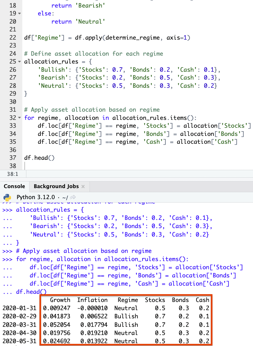
allocation_rules = {
    'Bullish': {'Stocks': 0.7, 'Bonds': 0.2, 'Cash': 0.1},
    'Bearish': {'Stocks': 0.2, 'Bonds': 0.5, 'Cash': 0.3},
    'Neutral': {'Stocks': 0.5, 'Bonds': 0.3, 'Cash': 0.2}
}

# Apply asset allocation based on regime
for regime, allocation in allocation_rules.items():
    df.loc[df['Regime'] == regime, 'Stocks'] = allocation['Stocks']
    df.loc[df['Regime'] == regime, 'Bonds'] = allocation['Bonds']
    df.loc[df['Regime'] == regime, 'Cash'] = allocation['Cash']

df.head()

Results

Based on our code and the synthetic data provided, we can see how the model chooses to allocate:

Conclusion

Regime-switching models are used for capturing the complex dynamics observed in financial markets and economic data.

Their ability to model changes in structural relationships makes them invaluable for forecasting, risk management, and structural analysis.

Implementing these models requires a solid understanding of statistical modeling techniques and computational methods, given the complexity of estimating model parameters and the non-linear nature of the regime transitions.