Factor Statistics


Factors in finance are systematic drivers of risk and return.
They help explain why assets move the way they do and why some earn higher returns or have higher risks than others.
They primary exist due to:
- risk compensation (which means they’re likely to endure and not merely be arbitraged out if discovered)
- psychological factors that make them persist (e.g., they can have long periods of underperformance)
We’re going to look at the popular factors studied both academically and by institutional investors.
What are they, what’s the idea behind them, and what are examples?
We then look at their risk, return, and correlations.
Key Takeaways – Factor Statistics
- Factors are systematic drivers of risk and return.
- Think of factors as the “DNA” behind asset performance.
- They explain why certain securities earn higher returns: compensation for risk or persistent behavioral biases.
- Core equity factors:
- Market – reward for taking broad equity risk.
- Size – small firms outperform large ones over time. (Note: This has mixed evidence over recent market history.)
- Value – cheap stocks beat expensive ones long-term.
- Momentum – winners keep winning short term.
- Profitability & Investment – efficient, profitable firms outperform.
- Reversal factors – capture short- and long-term mean reversion.
- Correlations are low, so combining factors improves diversification.
- Key insight: factor investing blends independent, persistent sources of return.
- Balance offense (momentum, value) and defense (quality, low volatility) to create steadier long-term performance.
- The ideal stock or investment to own, based on all the factors covered, would be a high-quality (strong assets, low debt), profitable company that invests conservatively/not overly aggressively, trades at a reasonable valuation (e.g., high earnings and operating cash flow relative to its price), has low volatility, and operates on a sustainable growth trajectory.
- Optionally, evidence of strong and consistent momentum.
- Essentially combining value, quality, momentum, and low-risk traits into one enduring business.
Fama-French Research Factors: Factor Return Statistics
1. Market (FF-MKT-RF)
This is the excess return of the overall stock market over the risk-free rate.
It’s the most popular factor in markets and is the fundamental idea behind buy-and-hold investing.
Companies produce earnings, which become capitalized in the share price or return to shareholders as dividends or distributions.
- Idea – Investors are rewarded for taking market risk rather than holding risk-free assets (like Treasury bills).
- Example – The classic “beta” in CAPM.
2. Size (FF3 or FF-SMB)
“Small Minus Big” is the return difference between small-cap and large-cap stocks.
- Idea – Historically, smaller companies tend to outperform larger ones over time.
- Reason – Smaller firms are riskier and less liquid, so investors demand higher returns.
3. Size (FF5 or FF-SMB5)
The size factor, as defined in the five-factor model, which adjusts for profitability and investment.
As we’ll see below, the FF5 size factor returns 40-50bps of extra return – for commensurate risk – relative to FF3.
- Difference – Slightly different construction from the FF3 version, but conceptually the same “small vs. big” idea.
4. Value (FF-HML)
“High Minus Low” or the return difference between value stocks (high book-to-market ratio) and growth stocks (low book-to-market).
- Idea – Value stocks outperform growth stocks long-term because growth stocks tend to underperform relative to expectations while value stocks represent what’s more tried and true.
- Example – Companies trading cheaply relative to fundamentals.
5. Momentum (FF-MOM)
The tendency of stocks that performed well recently to continue performing well in the short term.
- Idea – Markets underreact to information, so trends persist.
- Example – Buying recent winners and selling recent losers.
6. Profitability (FF-RMW)
“Robust Minus Weak” is the return spread between firms with high and low profitability.
- Idea – More profitable companies tend to generate higher returns.
- Why – Profitability signals economic strength and efficiency. Low profitability companies tend to have higher discounted growth, but it’s a matter of execution and their long duration gives them structurally higher risk.
7. Investment (FF-CMA)
“Conservative Minus Aggressive” is the return difference between firms that invest conservatively versus aggressively.
- Idea – Companies that reinvest less tend to outperform those that invest heavily.
- Why – Overinvestment often signals poor capital discipline.
8. Short-Term Reversal (FF-STREV)
Stocks that did poorly in the last month tend to rebound, and vice versa.
- Idea – Short-term overreactions or liquidity effects cause temporary mispricings.
- Example – A stock drops sharply due to forced selling or overreactions, then recovers.
9. Long-Term Reversal (FF-LTREV)
Stocks that have performed poorly over 3-5 years tend to outperform in the future.
- Idea – Long-term mean reversion, markets eventually correct overextended trends.
These factors describe systematic sources of risk and return that go beyond the market index.
Investors use them to explain portfolio performance or to construct factor-based (smart beta) strategies.
| Category | Factor | What It Captures |
| Market risk | Market (Rm-Rf) | Exposure to overall market returns |
| Size | SMB, SMB5 | Small vs. large companies |
| Value | HML | Cheap vs. expensive stocks |
| Momentum | MOM | Trend-following behavior |
| Profitability | RMW | Strong vs. weak earnings |
| Investment | CMA | Capital discipline |
| Reversals | STREV, LTREV | Short- and long-term mean reversion |
Factor Correlations: United States
| Factor | Key | Rm-Rf | SMB | SMB5 | HML | MOM | RMW | CMA | STREV | LTREV | Annualized Return | Annualized Standard Deviation |
|---|---|---|---|---|---|---|---|---|---|---|---|---|
| Market | FF-MKT-RF | 1.00 | 0.30 | 0.28 | -0.21 | -0.18 | -0.19 | -0.35 | 0.30 | -0.01 | 5.98% | 15.53% |
| Size (FF3) | FF-SMB | 0.30 | 1.00 | 0.98 | -0.14 | -0.05 | -0.41 | -0.17 | 0.17 | 0.25 | 1.35% | 10.53% |
| Size (FF5) | FF-SMB5 | 0.28 | 0.98 | 1.00 | 0.01 | -0.08 | -0.35 | -0.09 | 0.17 | 0.32 | 1.78% | 10.54% |
| Value | FF-HML | -0.21 | -0.14 | 0.01 | 1.00 | -0.19 | 0.09 | 0.68 | 0.02 | 0.52 | 2.92% | 10.33% |
| Momentum | FF-MOM | -0.18 | -0.05 | -0.08 | -0.19 | 1.00 | 0.08 | -0.01 | -0.31 | -0.09 | 6.13% | 14.53% |
| Profitability | FF-RMW | -0.19 | -0.41 | -0.35 | 0.09 | 0.08 | 1.00 | -0.00 | -0.08 | -0.26 | 3.00% | 7.70% |
| Investment | FF-CMA | -0.35 | -0.17 | -0.09 | 0.68 | -0.01 | -0.00 | 1.00 | -0.14 | 0.51 | 2.82% | 7.15% |
| Short Term Reversal | FF-STREV | 0.30 | 0.17 | 0.17 | 0.02 | -0.31 | -0.08 | -0.14 | 1.00 | 0.10 | 4.63% | 10.93% |
| Long Term Reversal | FF-LTREV | -0.01 | 0.25 | 0.32 | 0.52 | -0.09 | -0.26 | 0.51 | 0.10 | 1.00 | 2.22% | 9.16% |
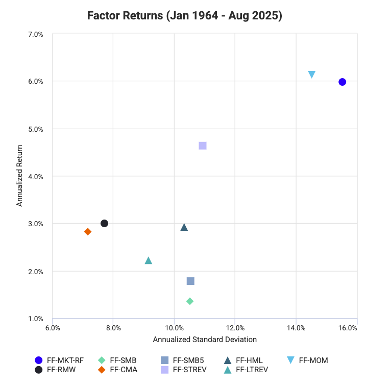
This table summarizes the relationships among key US equity risk factors from the Fama-French and related models, along with their long-term returns and volatility from 1964 to 2025.
First, why are the correlations so low?
Because they’re relative. You’re essentially taking one thing and subtracting the other to isolate it.
The market factor (FF-MKT-RF) delivers an annualized return of 5.98% with a 15.53% standard deviation, setting the benchmark for overall equity risk.
In other words, over more than 60 years of market history, the stock market has returned approximately 6% over T-bills (i.e., cash-like instruments).
The size factors (SMB, SMB5) show moderate correlation with the market (≈0.3) and obviously high correlation with each other (0.98), reflecting that small-cap stocks tend to move together. Their returns, around 1.3-1.8%, indicate a modest but persistent small-cap premium.
The value factor (HML), which contrasts cheap versus expensive stocks, has a low correlation with size and market risk, yielding a 2.92% annual return.
Momentum (MOM), the tendency for winners to keep winning, provides the strongest return at 6.13%, but with high volatility (14.53%) and negative/no correlation with most other factors, suggesting diversification benefits.
Profitability (RMW) and investment (CMA) are firm-quality dimensions: profitable, conservatively investing firms outperform. They show relatively low volatility (≈7%) and modest returns (3.0% and 2.82%).
Finally, reversal factors capture short-term corrections (STREV, 4.63%) and long-term mean reversion (LTREV, 2.22%). We can see that they’re only weakly correlated with other styles.
Overall, the results show that US equity returns are driven by multiple independent sources (market risk, size, value, momentum, and quality-related effects).
All contribute distinct patterns of risk and reward over time.
(How to find stocks that fit such factors? We recommend starting with a screening tool.)
Factor Performance

Factor Correlations: International Markets ex US
| Factor | Key | Rm-Rf | SMB | SMB5 | HML | MOM | RMW | CMA | Annualized Return | Annualized Standard Deviation |
|---|---|---|---|---|---|---|---|---|---|---|
| Market | FF-MKT-RF | 1.00 | -0.16 | -0.19 | -0.06 | -0.30 | -0.26 | -0.30 | 3.65% | 15.96% |
| Size (FF3) | FF-SMB | -0.16 | 1.00 | 0.99 | -0.09 | 0.13 | -0.02 | -0.07 | -0.44% | 6.68% |
| Size (FF5) | FF-SMB5 | -0.19 | 0.99 | 1.00 | 0.03 | 0.11 | -0.04 | 0.02 | 0.48% | 6.60% |
| Value | FF-HML | -0.06 | -0.09 | 0.03 | 1.00 | -0.27 | -0.42 | 0.64 | 4.53% | 8.09% |
| Momentum | FF-MOM | -0.30 | 0.13 | 0.11 | -0.27 | 1.00 | 0.35 | -0.05 | 7.36% | 11.70% |
| Profitability | FF-RMW | -0.26 | -0.02 | -0.04 | -0.42 | 0.35 | 1.00 | -0.34 | 3.37% | 4.75% |
| Investment | FF-CMA | -0.30 | -0.07 | 0.02 | 0.64 | -0.05 | -0.34 | 1.00 | 1.68% | 6.09% |
| Factor correlations and returns statistics from November 1990 to August 2025 | ||||||||||
This table summarizes the performance and relationships of international equity factors (excluding the US) from 1990 to 2025.
It’s also helpful to look outside the US to see how factors endure in other markets.
The market factor (FF-MKT-RF) shows an annualized return of 3.65% with a volatility of 15.96%. So, lower average equity premiums and similar risk levels compared to the US market.
The underperformance doesn’t necessarily mean extrapolating future underperformance.
The size factors (SMB and SMB5) are obviously highly correlated with each other (0.99) but weakly related to other styles. Their returns are minimal to slightly negative (-0.44% and 0.48%), indicating that the small-cap premium has been weak or absent in international markets during this period.
The value factor (HML) delivers a 4.53% annualized return with moderate risk (8.09%).
It’s strongly positively correlated with investment (0.64) and negatively with profitability (-0.42), reflecting how cheap stocks often invest conservatively and have lower profitability.
Momentum (MOM) remains the strongest performer, returning 7.36% annually, though with higher volatility (11.70%) and negative correlation with value (-0.27). This is better performance than in US markets.
Profitability (RMW) and investment (CMA) yield moderate returns (3.37% and 1.68%) with low volatility – i.e., capturing firm-quality and capital allocation effects across global markets.
Overall, these results show us that outside the US, momentum and value are – i.e., have been – the dominant rewarded factors, while size contributes little.
As we covered here, size has been less dominant in recent times as a driver.
International markets have displayed similar diversification patterns but weaker average risk premia than the US.
AQR Factors: Factor Return Statistics
This second table shows AQR-style factors, which are similar to the Fama-French factors but extended to include more refined and behaviorally informed styles.
These come from AQR’s public research (Asness, Frazzini, Pedersen, et al.), which builds on and refines the traditional factor framework.
Here’s what each one means:
1. Market (AQR-MKT-RF)
The excess return of the broad market portfolio over the risk-free rate.
- Idea – Same as the traditional market risk premium – investors expect higher returns for taking on market volatility.
- Example – The S&P 500’s return minus Treasury bill yields.
2. Size (AQR-SMB)
“Small Minus Big” — the difference in returns between small-cap and large-cap stocks.
- Idea – Small companies tend to outperform large ones over time because they’re less followed and riskier. Less institutional capital is after them, leaving a higher risk premium, at least in theory.
- Note – AQR’s construction may differ slightly (more diversified and global than Fama-French).
3. Value (AQR-HML)
“High Minus Low” or the return difference between value stocks (cheap based on fundamentals like book-to-market, earnings, or cash flow) and growth stocks (expensive).
As AQR founder Cliff Asness has written: “The value premium is a compensation for being uncomfortably right, at least for a while.”
- Idea – Value investing works long-term because investors often overpay for “exciting” growth stories and underpay for boring, steady businesses.
- Example – Buying companies trading at low price-to-book ratios.
4. Value (AQR-HML-DEV)
“Value-Developed” – a refined or region-specific version of the Value factor focusing on developed markets.
- Idea – Captures similar effects as HML but isolates them in developed economies, where accounting standards and market structures differ.
- Note – Its high correlation (0.79) with HML means it’s largely similar but measured differently (perhaps hedged for region, currency, or sector exposure).
5. Momentum (AQR-MOM)
The tendency for stocks that have recently gone up to keep going up in the short to medium term.
- Idea – Markets underreact to information, so recent winners continue to outperform losers for a while.
- Example – Buying top-performing stocks from the last 12 months and shorting the worst performers.
- Why it works – Behavioral biases and delayed price adjustments.
6. Quality (AQR-QMJ)
“Quality Minus Junk” – the return spread between high-quality and low-quality firms.
- What defines quality – Profitability, stability, growth, balance sheet strength, and sound corporate governance.
- Idea – Quality companies earn higher returns relative to their risk, despite being less volatile.
- Example – Owning companies with high ROE and low debt, while shorting those with weak profitability and high leverage.
7. Bet Against Beta (AQR-BAB)
A strategy that goes long low-beta stocks and shorts high-beta stocks, leveraging the low-beta portfolio to achieve market neutrality.
- Idea – Investors often overpay for high-volatility, “lottery-like” stocks, and underpay for boring, low-volatility ones.
- Result – Low-beta stocks tend to outperform on a risk-adjusted basis.
- Example – Preferring a stable utility company over a volatile biotech stock.
Summary Table
| Factor | Key | What It Captures | Core Idea |
| Market | AQR-MKT-RF | Market risk premium | Compensation for taking market-wide risk |
| Size | AQR-SMB | Small vs. large stocks | Smaller firms outperform long-term |
| Value | AQR-HML | Cheap vs. expensive | Value stocks outperform growth |
| Value (Developed) | AQR-HML-DEV | Regional value premium | Value effect within developed markets |
| Momentum | AQR-MOM | Trend persistence | Winners keep winning short-term |
| Quality | AQR-QMJ | Quality vs. junk | High-quality firms outperform low-quality ones |
| Bet Against Beta | AQR-BAB | Low-risk vs. high-risk | Low-beta stocks give better risk-adjusted returns |
Big Picture
These AQR factors reflect how systematic styles drive long-term returns across global equity markets:
- Market and Size are structural risks.
- Value and Momentum reflect behavioral inefficiencies.
- Quality and BAB reflect mispricing tied to investors’ preference for “exciting” or risky stocks.
AQR’s work builds a more diversified “style premia” model.
It emphasizes that good investing comes from harvesting multiple independent return sources, not just betting on the market.
Factor Correlations: United States
| Factor | Key | Rm-Rf | SMB | HML | HML-DEV | MOM | QMJ | BAB | Annualized Return | Annualized Standard Deviation |
|---|---|---|---|---|---|---|---|---|---|---|
| Market | AQR-MKT-RF | 1.00 | 0.31 | -0.23 | -0.06 | -0.19 | -0.53 | -0.09 | 5.62% | 15.61% |
| Size | AQR-SMB | 0.31 | 1.00 | -0.08 | 0.02 | -0.14 | -0.52 | -0.04 | 0.81% | 9.64% |
| Value | AQR-HML | -0.23 | -0.08 | 1.00 | 0.79 | -0.14 | -0.06 | 0.35 | 2.41% | 9.79% |
| Value | AQR-HML-DEV | -0.06 | 0.02 | 0.79 | 1.00 | -0.64 | -0.23 | 0.11 | 2.57% | 12.29% |
| Momentum | AQR-MOM | -0.19 | -0.14 | -0.14 | -0.64 | 1.00 | 0.31 | 0.21 | 6.77% | 14.24% |
| Quality | AQR-QMJ | -0.53 | -0.52 | -0.06 | -0.23 | 0.31 | 1.00 | 0.20 | 4.01% | 8.08% |
| Bet Against Beta | AQR-BAB | -0.09 | -0.04 | 0.35 | 0.11 | 0.21 | 0.20 | 1.00 | 8.87% | 11.24% |
| Factor correlations and returns statistics from January 1964 to July 2025 | ||||||||||
As Asness has stated, “Value and momentum, to me, are the two most interesting anomalies… The key is that they are very different from each other.”
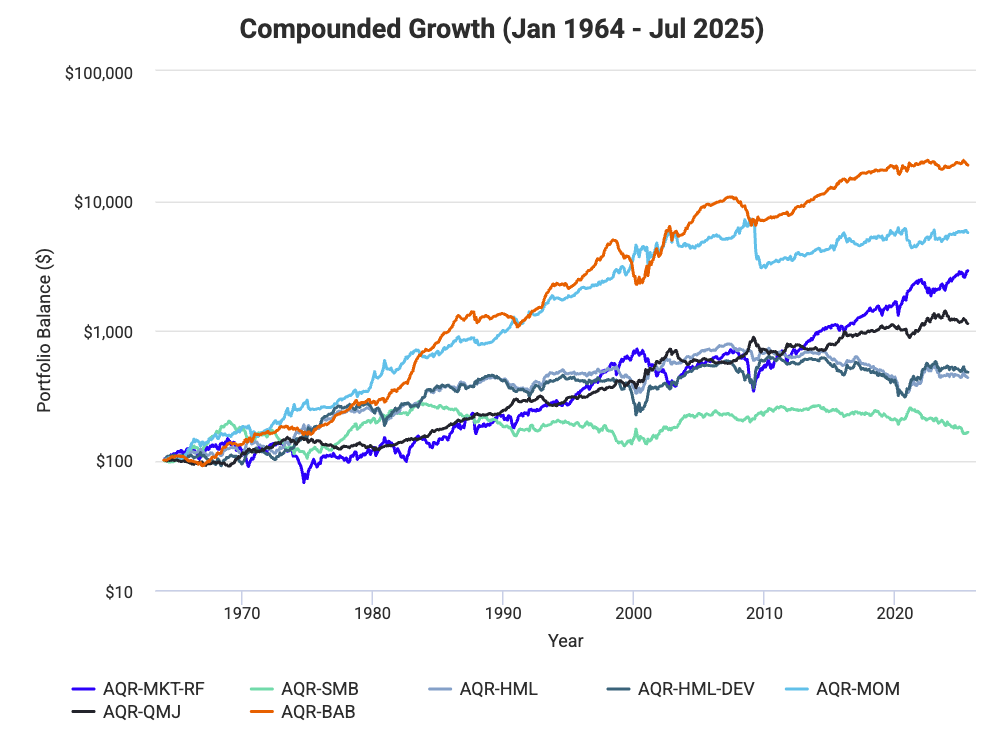
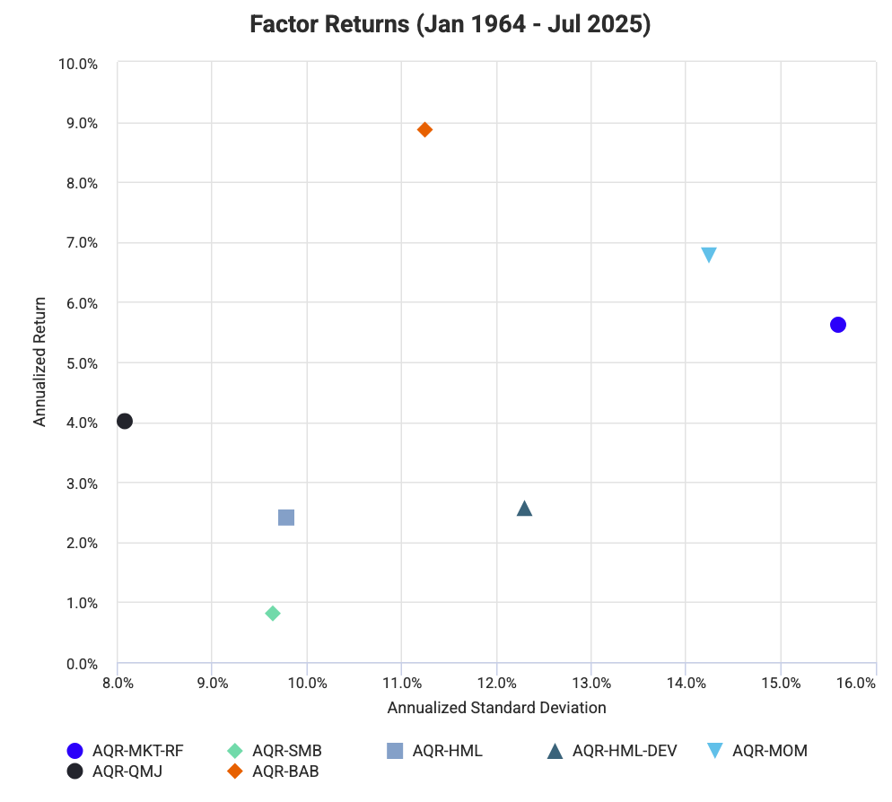
This table presents AQR’s US equity factor correlations and performance from 1964 to 2025.
These factors represent distinct, systematic sources of return used in multi-factor investing.
Together, they describe how market, style, and behavioral characteristics drive long-term equity performance.
The market factor (AQR-MKT-RF), which measures excess market return over the risk-free rate, shows a 5.62% annualized return with 15.61% volatility. It’s moderately correlated with the size factor (0.31) but negatively related to quality (-0.53). That suggests that quality stocks often underperform in strong markets.
The size factor (AQR-SMB), representing small versus large companies, delivers a modest 0.81% annualized return and moderate volatility (9.64%). Its negative correlation with quality (-0.52) and momentum (-0.14) indicates that smaller firms often lack stable earnings and consistent price trends.
The value factors (AQR-HML and AQR-HML-DEV) capture the premium for owning cheap stocks relative to expensive ones. They show strong internal correlation (0.79) but diverge in construction; the “DEV” version focuses on developed markets. Both generate annual returns near 2.4-2.6%, with the HML-DEV variant showing higher volatility (12.29%).
The momentum factor (AQR-MOM) is one of the strongest performers, with a 6.77% return and 14.24% standard deviation. Its correlations are largely negative with value and size, consistent with what we see with momentum’s tendency to favor growth-oriented, larger firms.
The quality factor (AQR-QMJ), or “Quality Minus Junk,” earns 4.01% annually with relatively low volatility (8.08%). It’s negatively correlated with the market and size. This reinforces the idea that high-quality firms (profitable, stable, and well-capitalized) can act as defensive assets during downturns. They’re better stores of value, in general.
Finally, Bet Against Beta (AQR-BAB), which favors low-volatility stocks over high-beta ones, yields 8.87% per year at 11.24% volatility. It’s positively correlated with value and quality. It reflects the long-term advantage of stable, lower-risk companies.
Overall, the AQR framework shows that returns stem from multiple independent drivers: market risk, company size, valuation, momentum, quality, and volatility.
Each contributes distinct risk premia. They combine to form a diversified, stronger equity return structure across market cycles.
As Asness writes: “Factors are not just anomalies; they’re part of the market’s structure. Factor investing is about capturing the risk premiums that have been shown to exist across markets and time.”
Factor Correlations: International Markets ex US
| Factor | Key | Rm-Rf | SMB | HML | HML-DEV | MOM | QMJ | BAB | Annualized Return | Annualized Standard Deviation |
|---|---|---|---|---|---|---|---|---|---|---|
| Market | AQR-MKT-RF | 1.00 | 0.31 | -0.23 | -0.06 | -0.19 | -0.53 | -0.09 | 5.62% | 15.61% |
| Size | AQR-SMB | 0.31 | 1.00 | -0.08 | 0.02 | -0.14 | -0.52 | -0.04 | 0.81% | 9.64% |
| Value | AQR-HML | -0.23 | -0.08 | 1.00 | 0.79 | -0.14 | -0.06 | 0.35 | 2.41% | 9.79% |
| Value | AQR-HML-DEV | -0.06 | 0.02 | 0.79 | 1.00 | -0.64 | -0.23 | 0.11 | 2.57% | 12.29% |
| Momentum | AQR-MOM | -0.19 | -0.14 | -0.14 | -0.64 | 1.00 | 0.31 | 0.21 | 6.77% | 14.24% |
| Quality | AQR-QMJ | -0.53 | -0.52 | -0.06 | -0.23 | 0.31 | 1.00 | 0.20 | 4.01% | 8.08% |
| Bet Against Beta | AQR-BAB | -0.09 | -0.04 | 0.35 | 0.11 | 0.21 | 0.20 | 1.00 | 8.87% | 11.24% |
| Factor correlations and returns statistics from January 1964 to July 2025 | ||||||||||
This table presents AQR’s international equity factor performance (excluding the US) from 1964 to 2025, capturing how different investment styles behave globally.
The market factor (AQR-MKT-RF) earns an annualized return of 5.62% with 15.61% volatility, setting the baseline for global equity risk.
The size factor (AQR-SMB) shows a small return of 0.81%, indicating the size premium is weak outside the US, though it remains moderately correlated with the market (0.31).
The value factors (AQR-HML and AQR-HML-DEV) produce returns of 2.41% and 2.57%, respectively, with a strong internal correlation of 0.79, showing consistent global value effects.
Momentum (AQR-MOM) stands out with a 6.77% return and higher volatility (14.24%). This reinforces its persistence across regions.
Quality (AQR-QMJ) earns 4.01% annually with lower volatility (8.08%) and negative correlation with market and size (i.e., defensive character).
Finally, Bet Against Beta (AQR-BAB) delivers a strong 8.87% return with 11.24% volatility, rewarding investors who favor low-risk, low-beta stocks.
Overall, international markets mirror US factor behavior: momentum, quality, and low beta deliver excess returns, while the size factor remains subdued.
These factors together can be used as a diversified global source of long-term equity risk premia.
What else has Cliff Asness said about factors?
Cliff Asness has the rare background of being both an academic and an institutional investor, and is one of the most knowledgeable about factor investing.
Some quotes:
“Factors are not magic; they’re not going to persist just because we want them to… They’ll persist if there’s a logical economic explanation for why they should persist.”
– Here, he cautions that the persistence of factors depends on their underlying economic rationale.
“If you believe in factors, then you should be allocating to them. It doesn’t matter if it’s ‘smart beta’ or ‘alternative risk premia’; call it whatever you like, just do it.”
– Asness encourages investors to embrace factor investing if they believe in its underlying principles, regardless of the terminology used.
“I don’t think there’s a lot of evidence that you can time these factors… the best way to implement factors is generally to run them at fairly constant risk weights.”
– Overall, he’s skeptical about the ability to time factors effectively and advocates for maintaining relatively constant risk exposures.
“If you’re a true believer in market efficiency, then you should just buy the market. But if you’re going to deviate, you should deviate on the side of the evidence.”
– This quote reflects his stance on market efficiency and the rationale for tilting towards evidence-backed factors.
“The best way to diversify is to diversify across different types of strategies, including different factors.”
– He emphasizes the importance of diversification across various factors to manage risk.
Alpha Architect Factors: Factor Return Statistics
Alpha Architect is a Pennsylvania-based Investment Adviser.
This shows Alpha Architect (AA) factors, which are similar in spirit to Fama-French and AQR factors but constructed independently using Alpha Architect’s data methodology and often with a more practitioner-oriented, rules-based approach.
Let’s go through each factor clearly:
1. Market (AA-MKT-RF)
The excess return of the overall market (stocks) over the risk-free rate (Treasury bills).
- Idea – This is the fundamental “market risk premium” – investors require compensation for holding risky assets rather than safe ones.
- Example – If the S&P 500 returned 10% and T-bills 3%, the market factor equals 7%.
- Annualized Return – 8.28%; quite consistent with long-run US equity premiums.
- Annualized Std. Dev.: 15.03%; typical for market-level volatility.
2. Size (AA-SMB)
“Small Minus Big”; performance spread between small-cap and large-cap stocks.
- Idea – Smaller companies have historically delivered higher returns, albeit with more volatility and liquidity risk.
- Behavior – Often countercyclical; small caps outperform when risk appetite is high.
- Annualized Return – 2.75%; modest, showing that the size effect has weakened in more recent decades.
- Annualized Std. Dev. – 11.15%
3. Value (AA-HML)
“High Minus Low” — difference between returns of cheap (high book-to-market or earnings-to-price) and expensive (low book-to-market) stocks.
- Idea – Value stocks outperform because investors overreact to bad news or avoid boring firms.
- Example – Buying low P/E industrials and shorting high P/E story stocks.
- Annualized Return – 1.87% – historically positive but more muted post-2000.
- Annualized Std. Dev. – 15.52% – value is volatile, as cheap stocks can stay cheap for long stretches.
4. Momentum (AA-MOM)
The return spread between recent winners and losers.
- Idea – Stocks with strong recent performance tend to continue that trend over the next 6-12 months.
- Why it works – Behavioral biases (investor underreaction, herding) and slow information diffusion.
- Notable correlation – Strongly positive (0.73) with Quality (QMJ); likely because quality firms often maintain upward momentum.
- Annualized Return – 2.26%
- Annualized Std. Dev. – 15.46%
5. Quality (AA-QMJ)
“Quality Minus Junk”; the difference in returns between high-quality firms (strong profitability, low leverage, stable earnings) and low-quality firms.
- Idea – High-quality companies generate better risk-adjusted returns because investors underestimate their consistency.
- Alpha Architect’s emphasis – They often define quality using variables like ROE, earnings stability, and leverage, following a “quant value + quant quality” philosophy.
- Annualized Return – 1.15%
- Annualized Std. Dev. – 8.87% – relatively low risk compared to others.
Summary Table
| Factor | Key | What It Captures | Core Idea |
| Market | AA-MKT-RF | Market risk premium | Return from broad equity exposure |
| Size | AA-SMB | Small vs. large stocks | Small companies outperform large ones |
| Value | AA-HML | Cheap vs. expensive stocks | Value stocks outperform growth stocks |
| Momentum | AA-MOM | Recent winners vs. losers | Price trends persist short-term |
| Quality | AA-QMJ | Strong vs. weak fundamentals | High-quality firms outperform low-quality ones |
How Alpha Architect’s Factors Differ
Alpha Architect’s philosophy puts an emphasis on practitioner-grade transparency and strong data construction rather than theoretical elegance.
How is it different than AQR or Fama-French?
- They try to use more replicable signals, often grounded in public data only.
- They emphasize implementation feasibility. They focus on investable portfolios rather than academic ones.
- Their factors cover a shorter window (1992-2024), which might make them more relevant to modern market behavior.
In short, Alpha Architect’s factors capture the same broad ideas (market, size, value, momentum, and quality) but with a modern, data-clean, practitioner-friendly twist.
Their approach tends to appeal to traders/investors who want to apply systematic style investing in real-world portfolios, and not just study it academically (like with Fama-French, in particular).
Factor Correlations: United States
| Factor | Key | Rm-Rf | SMB | HML | MOM | QMJ | Annualized Return | Annualized Standard Deviation |
|---|---|---|---|---|---|---|---|---|
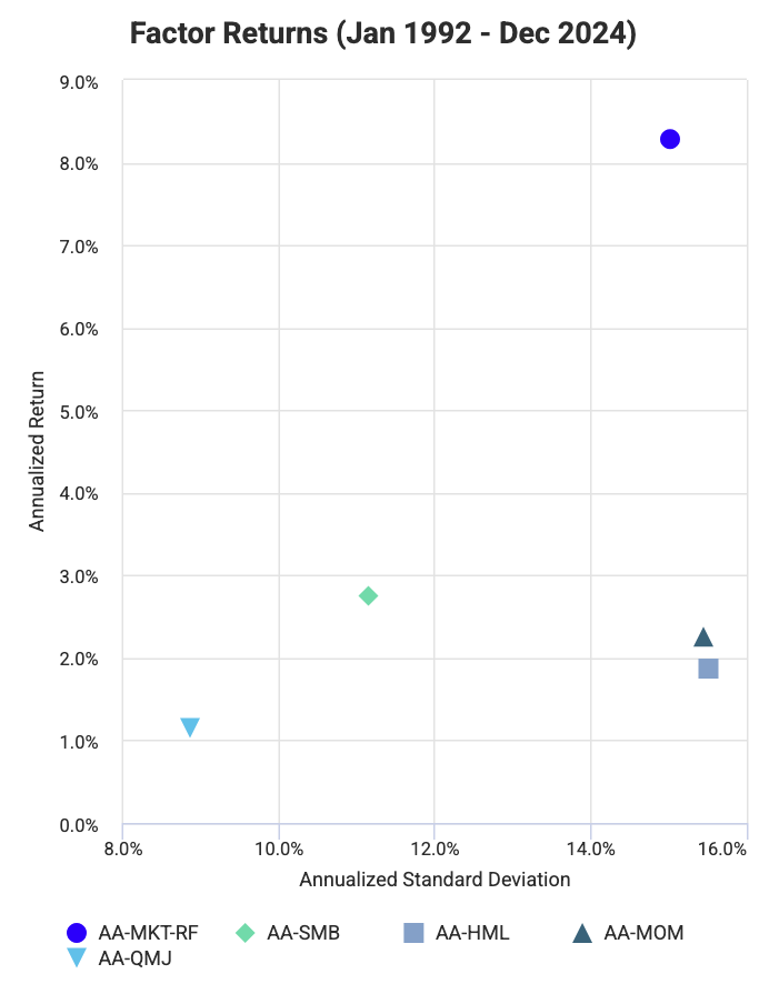
| Market | AA-MKT-RF | 1.00 | 0.27 | -0.32 | -0.25 | -0.34 | 8.28% | 15.03% |
| Size | AA-SMB | 0.27 | 1.00 | -0.27 | -0.19 | -0.40 | 2.75% | 11.15% |
| Value | AA-HML | -0.32 | -0.27 | 1.00 | -0.30 | 0.12 | 1.87% | 15.52% |
| Momentum | AA-MOM | -0.25 | -0.19 | -0.30 | 1.00 | 0.73 | 2.26% | 15.46% |
| Quality | AA-QMJ | -0.34 | -0.40 | 0.12 | 0.73 | 1.00 | 1.15% | 8.87% |
| Factor correlations and returns statistics from January 1992 to December 2024 | ||||||||
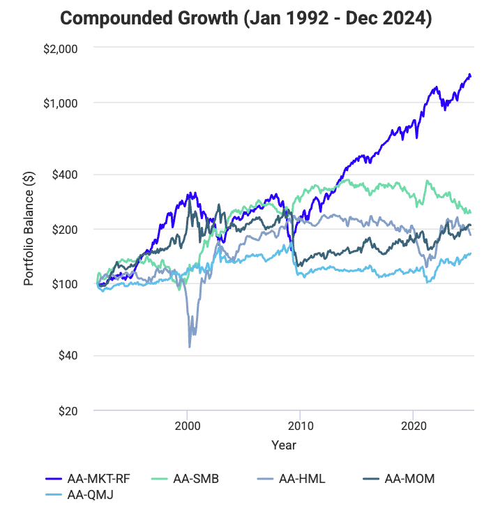
In this table we summarize Alpha Architect’s US factor correlations and performance between 1992 and 2024.
The framework looks at five key dimensions of equity risk and behavior (market, size, value, momentum, and quality), which together explain the majority of systematic variation in US stock returns.
The market factor (AA-MKT-RF) delivers 8.28% annualized return with 15.03% volatility, higher than the historical equity risk premium. It shows modest correlation with size (0.27) but negative links to value, momentum, and quality (-0.32 to -0.34), implying that these defensive or contrarian strategies often outperform when broad markets lag.
The size factor (AA-SMB), which captures the small-cap premium, earns 2.75% per year at 11.15% volatility. It’s negatively correlated with most factors, especially quality (-0.40), as smaller companies often have lower profitability and less stable fundamentals.
The value factor (AA-HML), or the return spread between cheap and expensive stocks, earns 1.87% annually with high volatility (15.52%). Its weak correlation with other factors shows that valuation-based strategies provide independent diversification benefits.
Momentum (AA-MOM), which rewards stocks that have recently performed well, posts 2.26% annual returns with similar volatility (15.46%). It’s positively correlated with quality (0.73), which you can argue suggests that stronger, higher-quality firms often see sustained performance trends.
Finally, the quality factor (AA-QMJ), or “Quality Minus Junk,” earns a lower 1.15% return but with the lowest volatility (8.87%). Quality’s negative correlation with the market (-0.34) and size (-0.40) confirms its defensive tilt: high-quality stocks tend to outperform in risk-off periods or downturns.
Overall, Alpha Architect’s factors show that these multiple, distinct sources of return coexist in US equities.
Market exposure remains the primary driver, but systematic styles, especially momentum and quality, offer good diversification.
This blend of risk-based and behavioral effects gives an evidence-based foundation for systematic portfolio construction across different market environments.
Factor Correlations: International Markets ex US
| Factor | Key | Rm-Rf | SMB | HML | MOM | QMJ | Annualized Return | Annualized Standard Deviation |
|---|---|---|---|---|---|---|---|---|
| Market | AA-MKT-RF | 1.00 | -0.04 | -0.24 | -0.27 | -0.42 | 3.24% | 16.55% |
| Size | AA-SMB | -0.04 | 1.00 | 0.01 | -0.21 | -0.16 | 0.15% | 6.21% |
| Value | AA-HML | -0.24 | 0.01 | 1.00 | -0.28 | -0.07 | 4.14% | 7.85% |
| Momentum | AA-MOM | -0.27 | -0.21 | -0.28 | 1.00 | 0.71 | 3.71% | 14.12% |
| Quality | AA-QMJ | -0.42 | -0.16 | -0.07 | 0.71 | 1.00 | 2.59% | 7.66% |
| Factor correlations and returns statistics from January 1992 to December 2024 | ||||||||
This table summarizes Alpha Architect’s international (ex-US) equity factors from 1992 to 2024.
It shows how global style premiums differ from US markets.
The market factor (AA-MKT-RF) delivers a 3.24% annualized return with high volatility (16.55%), showing more modest risk-adjusted returns abroad.
The size factor (AA-SMB) is weak, with only 0.15% return, showing little small-cap premium internationally. This dovetails with the idea that the size factor has eroded in recent market history.
The value factor (AA-HML) performs best, earning 4.14% annually at moderate volatility (7.85%).
Momentum (AA-MOM) and quality (AA-QMJ) also produce positive returns of 3.71% and 2.59%, respectively, with strong correlation (0.71). Again, this shows that profitable, high-quality firms often sustain performance trends.
Negative correlations between market and defensive factors (quality = -0.42) confirm their protective role during downturns.
Overall, global markets outside the US show – or at least have shown – lower market returns but consistent strength in value, momentum, and quality, which emphasizes their importance in diversified international portfolios.
q-Factors: Factor Return Statistics
Now we’re going to look at the “q-Factors”, developed by Hou, Xue, and Zhang (HXZ), often referred to as the q-factor model.
This model is an alternative to Fama-French and AQR frameworks and is grounded more directly in corporate finance theory rather than purely empirical patterns.
The goal is to explain stock returns using firm-level economic fundamentals (specifically investment and profitability) rather than statistical or behavioral constructs.
Let’s go through each factor in clear terms:
1. Market (Q-MKT-RF)
The usual thing that everyone goes after – excess return of the stock market over the risk-free rate.
- Purpose – Captures broad market exposure, the same “equity risk premium” used across all factor models.
- Idea – Investors are compensated for taking systematic market risk.
- Annualized Return – 6.08%
- Annualized Std. Dev. – 15.82%
2. Size (Q-ME)
The return spread between small and large firms.
(“ME” stands for market equity.)
- Idea – Small firms are riskier and less liquid, which earns them a higher long-term return.
- Theoretical Link – Smaller firms often face higher financing constraints, making their risk premium higher in the q-model framework.
- Annualized Return – 2.40%
- Annualized Std. Dev. – 10.66%
3. Investment (Q-I/A)
“Investment-to-Assets”, i.e., the difference between firms that invest conservatively and those that invest aggressively.
- Idea – Firms that invest less (conservatively) tend to outperform those that invest heavily.
- Why – High investment usually reflects high optimism or low required returns, which leads to lower subsequent stock returns.
- Economic Interpretation – Overinvestment tends to be associated with overvaluation.
- Annualized Return – 3.92%
- Annualized Std. Dev. – 7.15% (quite low; this is a stable factor)
4. Return on Equity (Q-ROE)
The difference in returns between firms with high and low profitability (measured by Return on Equity).
- Idea – Profitable firms tend to have higher expected returns because profitability signals strong future cash flows and operational efficiency.
- Link to Fama-French – Similar to the RMW (Robust Minus Weak) profitability factor, but measured directly as ROE.
- Annualized Return – 6.23%
- Annualized Std. Dev. – 9.03%
5. Expected Growth (Q-EG)
The expected growth in future firm profitability or investment, estimated from firm-level fundamentals.
- Idea – Firms with high expected growth in productivity or earnings tend to earn higher returns.
- Why it matters – It connects current valuation to forward-looking fundamentals. It’s a cleaner link between market prices and expected economic output.
- Correlation Insight – Strong positive correlation (0.53) with ROE. Firms with strong profitability often have higher expected growth.
- Annualized Return – 9.42%
- Annualized Std. Dev. – 7.26%
Summary Table
| Factor | Key | What It Captures | Core Idea |
| Market | Q-MKT-RF | Market risk premium | Compensation for bearing market risk |
| Size | Q-ME | Small vs. large firms | Small firms earn a risk premium for higher constraints |
| Investment | Q-I/A | Conservative vs. aggressive investment | Firms investing less outperform those investing more |
| Profitability | Q-ROE | High vs. low return on equity | Profitability predicts higher future returns |
| Expected Growth | Q-EG | Expected future productivity growth | Firms with strong growth expectations outperform |
How the Q-Factor Model Differs
Compared with Fama-French or AQR models, the HXZ q-factor model is:
- Economically grounded – Built from real firm behavior (investment and profitability decisions) rather than empirical anomalies.
- Simpler – Fewer factors (four or five, depending on specification). They can explain returns nearly as well as more complex models. (If anything, there are diminishing returns.)
- Forward-looking – Focuses on expected future growth and profitability, not backward-looking valuation ratios.
- Cleaner mathematically – Ties directly to firm-level investment theory. Expected returns are higher when firms face higher costs of capital and lower when they overinvest.
In short
The q-factors give you the fundamental economic logic of stock returns:
- Firms that are small, conservative in investment, profitable, and expected to grow efficiently tend to outperform.
- It’s a model that connects financial economics (firm decisions) with asset pricing. Offers a more structural alternative to Fama-French or behavioral factor models.
Factor Correlations: United States
| Factor | Key | Rm-Rf | ME | I/A | ROE | EG | Annualized Return | Annualized Standard Deviation |
|---|---|---|---|---|---|---|---|---|
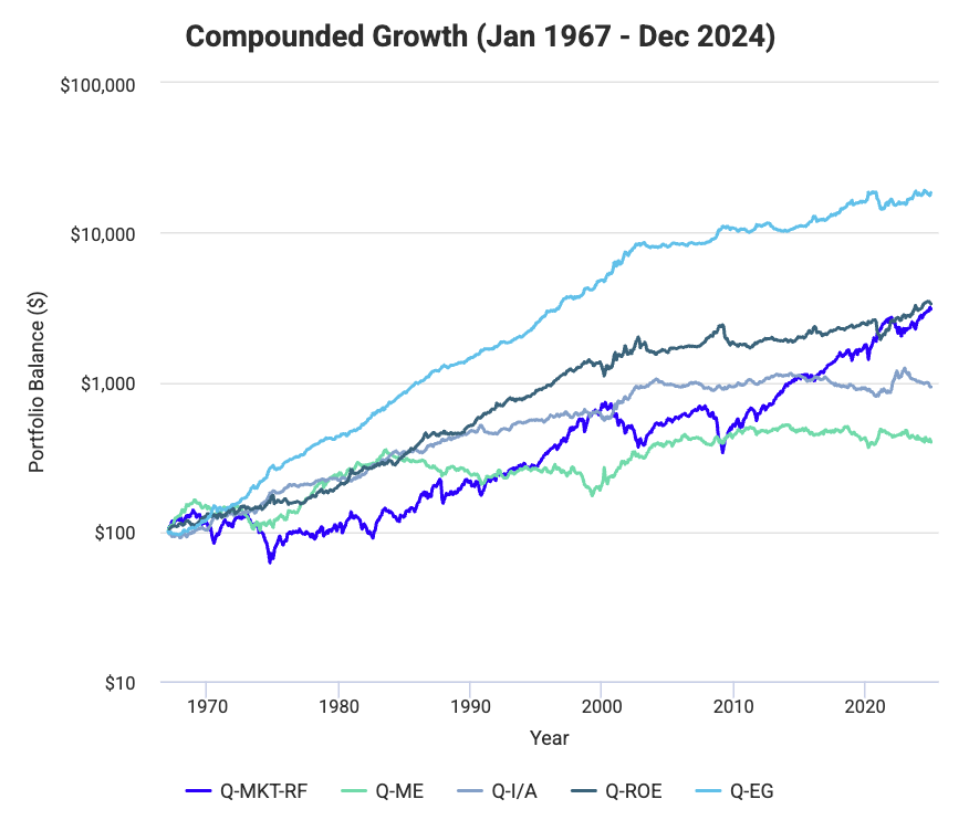
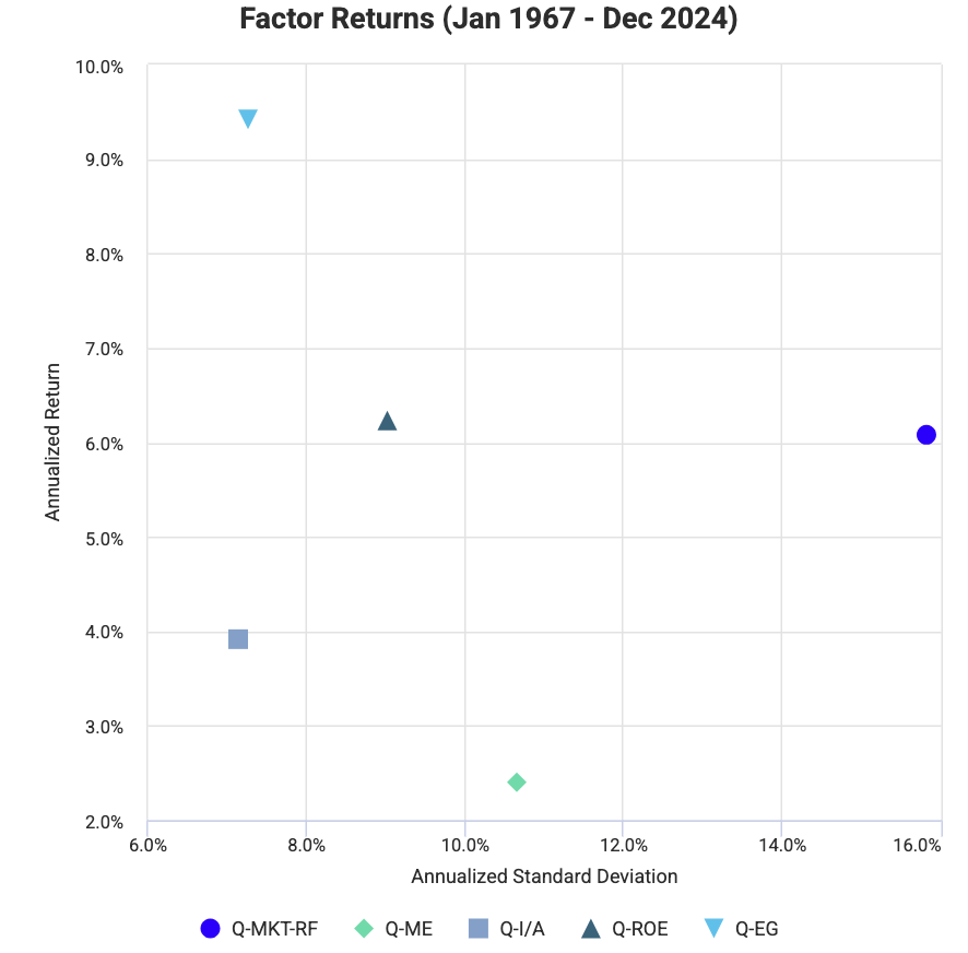
| Market | Q-MKT-RF | 1.00 | 0.28 | -0.35 | -0.22 | -0.43 | 6.08% | 15.82% |
| Size | Q-ME | 0.28 | 1.00 | -0.09 | -0.32 | -0.41 | 2.40% | 10.66% |
| Investment | Q-I/A | -0.35 | -0.09 | 1.00 | 0.05 | 0.18 | 3.92% | 7.15% |
| Return on Equity | Q-ROE | -0.22 | -0.32 | 0.05 | 1.00 | 0.53 | 6.23% | 9.03% |
| Expected Growth | Q-EG | -0.43 | -0.41 | 0.18 | 0.53 | 1.00 | 9.42% | 7.26% |
| Factor correlations and returns statistics from January 1967 to December 2024 | ||||||||
So here we summarize the US q-factor model, developed by Hou, Xue, and Zhang, which explains stock returns using firm-level fundamentals grounded in investment and profitability theory. The data covers 1967-2024 and highlights how firm behavior, not just valuation, drives long-term performance.
The market factor (Q-MKT-RF) delivers a 6.08% annualized return with 15.82% volatility, representing the equity risk premium. It’s moderately correlated with size (0.28) but negatively related to investment (-0.35) and expected growth (-0.43), showing that high-growth or low-investment firms tend to outperform when market returns are weaker.
The size factor (Q-ME) earns a 2.40% return at 10.66% volatility, reflecting a persistent but moderate small-cap premium. Its negative correlation with profitability (-0.32) and growth (-0.41) implies that smaller firms often have lower earnings quality and less predictable growth.
The investment factor (Q-I/A), which measures the return spread between firms that invest conservatively versus aggressively, earns 3.92% annually with low volatility (7.15%). This supports the view that companies engaging in heavy investment tend to be overvalued, while more cautious investors earn higher long-run returns.
The profitability factor (Q-ROE) delivers 6.23% with 9.03% volatility and correlates strongly with expected growth (0.53), indicating that profitable firms often sustain higher growth expectations.
Finally, the expected growth factor (Q-EG) provides the highest return (9.42%) and the lowest correlation with market risk (-0.43), suggesting that markets reward firms with consistent forward-looking profitability and efficient capital use.
Overall, the Q-factors provide an economically grounded view of returns: firms with high profitability, conservative investment, and strong growth expectations consistently outperform, linking asset pricing directly to real business fundamentals rather than statistical anomalies.
Factor Correlations: International Markets ex US
| Factor | Key | Rm-Rf | ME | I/A | ROE | EG | Annualized Return | Annualized Standard Deviation |
|---|---|---|---|---|---|---|---|---|
| Market | Q-MKT-RF | 1.00 | 0.28 | -0.35 | -0.22 | -0.43 | 6.08% | 15.82% |
| Size | Q-ME | 0.28 | 1.00 | -0.09 | -0.32 | -0.41 | 2.40% | 10.66% |
| Investment | Q-I/A | -0.35 | -0.09 | 1.00 | 0.05 | 0.18 | 3.92% | 7.15% |
| Return on Equity | Q-ROE | -0.22 | -0.32 | 0.05 | 1.00 | 0.53 | 6.23% | 9.03% |
| Expected Growth | Q-EG | -0.43 | -0.41 | 0.18 | 0.53 | 1.00 | 9.42% | 7.26% |
| Factor correlations and returns statistics from January 1967 to December 2024 | ||||||||
This table summarizes the q-factor model for international markets (excluding the US) from 1967 to 2024.
So how do firm fundamentals drive global equity returns?
The market factor (Q-MKT-RF) provides a 6.08% annualized return with 15.82% volatility, serving as the baseline for global equity risk.
The size factor (Q-ME) earns 2.40% annually, showing that smaller firms continue to command a modest premium, though less pronounced than in US markets.
The investment factor (Q-I/A) yields 3.92% with very low volatility (7.15%). So, as found before, firms with conservative investment policies outperform those expanding aggressively.
The profitability factor (Q-ROE) generates 6.23% at 9.03% volatility, closely tied to expected growth (Q-EG), which shows a strong 0.53 correlation and the highest return (9.42%).
So, we find that these results show that across global markets, profitability, prudent investment, and forward-looking growth expectations are the best drivers of returns.
Overall, the q-factor model’s strength is linking stock performance to real economic fundamentals.
These end up consistent across both US and international markets.
Fixed Income Factors: Factor Return Statistics
Now we’re going to look at fixed income (bond market) risk factors, which explain how bond returns vary based on changes in:
- interest rates,
- credit spreads, and
- duration exposure
Unlike the equity factors we shared earlier (which explain stock returns), these describe the main drivers of bond and credit portfolio performance.
Let’s go through each:
1. Intermediate Term Rate Risk (ITRM)
The return sensitivity to changes in intermediate-term Treasury yields (typically around 5–10 years).
- Idea – Bonds with intermediate maturities gain when yields fall and lose when yields rise.
- Interpretation – Captures interest rate duration risk in the mid-part of the yield curve.
- Example – A 7-year Treasury bond will move moderately in response to rate changes compared to short-term or long-term bonds.
- Annualized Return – 1.10%
- Annualized Std. Dev. – 4.26%
- Correlation – Strongly correlated (0.73) with long-term rate risk, both are rate-driven, not credit-driven.
2. Long Term Rate Risk (LTRM)
The return sensitivity to changes in long-term Treasury yields (typically 20+ years).
- Idea – Captures the duration risk at the far end of the yield curve.
- Why it matters – Long-term bonds are far more volatile because their prices react strongly to changes in long-term rates.
- Example – A 30-year Treasury bond’s price jumps sharply when long rates fall.
- Annualized Return – 0.51%
- Annualized Std. Dev. – 9.22%; much higher volatility, as expected for longer duration exposure.
- Correlation – 0.73 with ITRM. Both move together due to yield curve shifts. The further along the curve you get, the more correlated the movement.
3. Credit Risk (CDTA)
The excess return of corporate bonds over risk-free Treasuries of the same maturity.
- Idea – Traders/investors demand a premium for bearing the risk that a company might default or its credit quality might deteriorate.
- Interpretation – Captures the broad investment-grade credit spread risk.
- Example – The difference in yield between AAA or BBB corporate bonds and Treasuries.
- Annualized Return – 2.22%
- Annualized Std. Dev. – 7.04%
- Correlation – Highly correlated (0.87) with High Yield Credit Risk. Both move with the broader credit cycle.
4. High Yield Credit Risk (HY)
The excess return of high yield (junk) bonds over Treasuries.
- Idea – Reflects exposure to lower-quality corporate debt, which is more sensitive to economic cycles and default risk.
- Example – Bonds rated below BBB that behave more like equities during risk-on/risk-off periods.
- Annualized Return – 4.30%; the highest of the group, reflecting the higher yield premium for taking credit risk.
- Annualized Std. Dev. – 6.22%
- Correlation – 0.87 with Credit Risk. Both represent exposure to corporate bond spreads, but HY captures deeper, more cyclical risk.
Summary Table
| Factor | Key | What It Captures | Core Idea |
| Intermediate Term Rate Risk | ITRM | Mid-curve duration exposure | Bond prices move with intermediate rate changes |
| Long Term Rate Risk | LTRM | Long-duration interest rate exposure | Long-term bonds are highly sensitive to rate shifts |
| Credit Risk | CDTA | Investment-grade credit spread | Extra return for lending to corporations over governments |
| High Yield Credit Risk | HY | Non-investment-grade credit spread | Higher yield premium for taking on default risk |
How to Think About These Factors
Each of these factors represents a core dimension of bond return:
- Rate risk (ITRM, LTRM) – Driven by changes in Treasury yields and duration exposure.
- Credit risk (CDTA, HY) – Driven by changes in credit spreads and default risk.
Together, they capture nearly all systematic risks in fixed income portfolios.
- Government bond portfolios load mostly on ITRM and LTRM.
- Corporate bond portfolios load on CDTA (investment grade) or HY (high yield).
- Multi-sector fixed income portfolios are combinations of all four.
In short
These fixed income factors explain why bond returns move:
- Rates fall -> positive ITRM/LTRM returns.
- Credit spreads tighten -> positive CDTA/HY returns.
- Rates rise or credit spreads widen -> negative factor returns.
They form the bond equivalent of Fama-French factors, so essentially they summarize systematic risk premia in fixed income markets.
Factor Correlations: United States
| Factor | Key | ITRM | LTRM | CDT | HY | Annualized Return | Annualized Standard Deviation |
|---|---|---|---|---|---|---|---|
| Intermediate Term Rate Risk | ITRM | 1.00 | 0.73 | 0.06 | 0.00 | 1.10% | 4.26% |
| Long Term Rate Risk | LTRM | 0.73 | 1.00 | -0.03 | -0.11 | 0.51% | 9.22% |
| Credit Risk | CDTA | 0.06 | -0.03 | 1.00 | 0.87 | 2.22% | 7.04% |
| High Yield Credit Risk | HY | 0.00 | -0.11 | 0.87 | 1.00 | 4.30% | 6.22% |
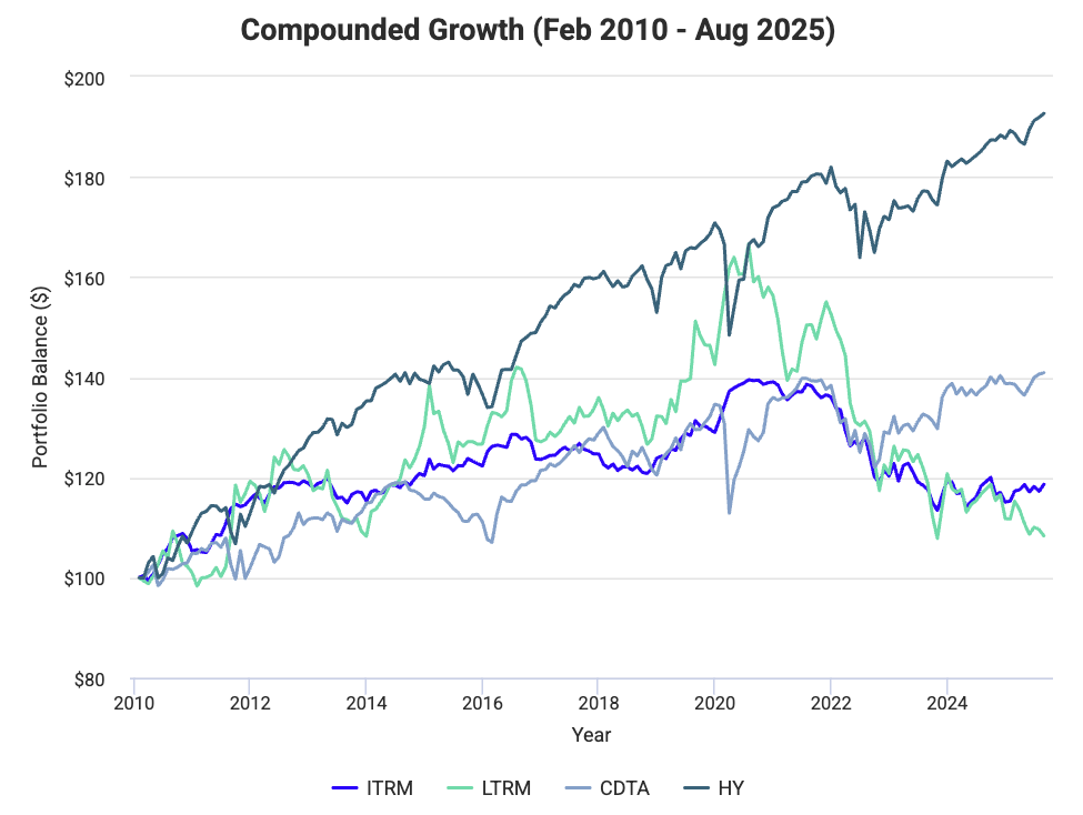
| Factor correlations and returns statistics from February 2010 to August 2025 | |||||||
This table presents the main US fixed income risk factors from 2010 to 2025.
They show how interest rate and credit dynamics drive bond market performance.
The Intermediate-Term Rate Risk (ITRM) factor, representing exposure to mid-maturity Treasuries, shows an annualized return of 1.10% with low volatility (4.26%).
It’s strongly correlated (0.73) with Long-Term Rate Risk (LTRM), so there’s shared sensitivity to yield curve movements. LTRM, tied to long-duration bonds, has higher volatility (9.22%) and a smaller return (0.51%), consistent with the greater price swings of long-dated securities.
The Credit Risk (CDTA) factor captures excess returns of investment-grade corporate bonds over Treasuries, earning 2.22% annually with 7.04% volatility.
CDTA is highly correlated (0.87) with High Yield Credit Risk (HY), which represents exposure to lower-quality, higher-yield bonds.
HY delivers the strongest return at 4.30%, compensating investors for greater default risk, though with moderate volatility (6.22%).
Overall, correlations show that rate risk (ITRM, LTRM) is largely distinct from credit risk (CDTA, HY), so this can provide diversification across bond portfolios.
Overall, these fixed income factors show the trade-off between interest rate sensitivity and credit exposure.

How to Turn Factors Into a Portfolio
Adding factors to a portfolio is essentially about building exposure to the underlying drivers of return rather than focusing on individual securities.
So they’re fundamentally about persistent, systematic sources of risk and reward that we’ve covered (e.g., value, momentum, size, quality, or low volatility) that can be combined to create a more balanced and stronger portfolio.
Here’s how to do it thoughtfully and effectively.
1. Understand what you’re targeting
Each factor represents a unique return pattern.
- Value – Stocks that are cheap relative to fundamentals (e.g., book-to-price, P/E).
- Momentum – Stocks that have recently performed well.
- Size – Small-cap stocks that tend to outperform large caps over time.
- Quality/Profitability – Firms with strong balance sheets and steady earnings.
- Low Volatility or BAB (Bet Against Beta) – Stocks with stable price movements that earn excess risk-adjusted returns.
The first step is deciding which factors align with your trading or investment philosophy.
For example, some people like value. They feel much more comfortable with 10x P/E securities that 50x growth names.
Others like quality, such as a 15x P/E stock with low debt and strong assets.
For instance, a long-term investor looking for stable compounding might focus on value, quality, and low volatility, while a more tactical trader might add momentum for shorter-term performance boosts.
2. Structure your factor exposures
To isolate a factor, you typically go long the securities with high exposure to that factor and short those with low exposure.
This creates a market-neutral factor portfolio that captures the pure effect of the characteristic.
For example:
- Long high-value stocks, short expensive stocks -> captures the value premium.
- Long recent outperformers, short recent underperformers -> captures momentum.
- Long high-quality companies, short low-quality ones -> captures quality.
This “long–short” approach nets out broad market risk and focuses your return on the factor itself, rather than general market moves.
Long-Only Approaches
If you prefer a long-only implementation, you can tilt your portfolio weights toward the desired factors.
For instance, overweighting high-value or high-momentum stocks and underweighting their opposites.
3. Decide how to weight factors
There are several ways to combine factors:
- Equal-weighted – Simple and balanced. Each factor contributes equally (e.g., 20% each to value, momentum, quality, size, and low volatility).
- Risk-parity weighting – Allocates more to low-volatility factors so that each contributes the same level of portfolio risk.
- Performance-based weighting – Allocates more to factors currently performing well (momentum in factors themselves).
Risk parity is generally best for diversification since some factors (like momentum) are more volatile than others (like value or quality).
Adjusting for volatility, each factor has a similar impact on overall risk.
4. Example: diversified factor portfolio
Let’s say you want a five-factor equity portfolio. You could structure it as follows (market-neutral setup):
| Factor | Long Exposure | Short Exposure | Weight |
| Value | Undervalued stocks | Expensive stocks | 20% |
| Momentum | Recent outperformers | Recent underperformers | 20% |
| Quality | Profitable, low-debt firms | Weak balance sheets | 20% |
| Low Volatility (BAB) | Stable, low-beta stocks | High-beta stocks | 20% |
| Size | Small-cap stocks | Large-cap stocks | 20% |
This portfolio would be roughly market-neutral, long and short positions offset general market exposure, but diversified across independent styles.
If you prefer a long-only variant, you could instead overweight these characteristics in a broad equity portfolio (for example, using ETFs like VLUE, MTUM, QUAL, and USMV in equal proportion).
5. Monitor and rebalance
Factor exposures shift over time as markets change.
Rebalance periodically (quarterly or semiannually) to maintain intended exposure, and watch correlations: when factors start moving together, diversification benefits shrink.
Putting it all together
A well-designed factor portfolio combines low-correlated, high-quality factor premia using relatively balanced weighting – e.g., risk-adjusted weighting.
Going long strong expressions of each and short their opposites, or tilting exposures in a long-only structure, you can achieve a blend of defensive and return-seeking characteristics.
The result: a portfolio that’s not dependent on one market environment but instead earns steady, repeatable excess returns across cycles.
Appendix
Factor Correlations: Fama-French + AQR
Factor Correlations
| Factor | FF-MKT-RF | AQR-MKT-RF | FF-SMB | FF-SMB5 | AQR-SMB | FF-HML | AQR-HML | AQR-HML-DEV | FF-MOM | AQR-MOM | FF-RMW | FF-CMA | FF-STREV | FF-LTREV | AQR-QMJ | AQR-BAB | Annualized Return | Annualized Standard Deviation |
|---|---|---|---|---|---|---|---|---|---|---|---|---|---|---|---|---|---|---|
| FF-MKT-RF | 1.00 | 1.00 | 0.30 | 0.28 | 0.31 | -0.21 | -0.24 | -0.07 | -0.17 | -0.19 | -0.19 | -0.35 | 0.30 | -0.01 | -0.52 | -0.09 | 5.96% | 15.54% |
| AQR-MKT-RF | 1.00 | 1.00 | 0.30 | 0.28 | 0.31 | -0.20 | -0.23 | -0.06 | -0.18 | -0.19 | -0.20 | -0.35 | 0.31 | -0.00 | -0.53 | -0.09 | 5.62% | 15.61% |
| FF-SMB | 0.30 | 0.30 | 1.00 | 0.98 | 0.96 | -0.15 | -0.11 | -0.06 | -0.05 | -0.06 | -0.41 | -0.17 | 0.17 | 0.25 | -0.49 | -0.07 | 1.29% | 10.52% |
| FF-SMB5 | 0.28 | 0.28 | 0.98 | 1.00 | 0.96 | 0.01 | 0.03 | 0.06 | -0.08 | -0.09 | -0.35 | -0.09 | 0.17 | 0.32 | -0.48 | -0.01 | 1.70% | 10.53% |
| AQR-SMB | 0.31 | 0.31 | 0.96 | 0.96 | 1.00 | -0.09 | -0.08 | 0.02 | -0.13 | -0.14 | -0.38 | -0.17 | 0.25 | 0.25 | -0.52 | -0.04 | 0.81% | 9.64% |
| FF-HML | -0.21 | -0.20 | -0.15 | 0.01 | -0.09 | 1.00 | 0.95 | 0.79 | -0.19 | -0.18 | 0.09 | 0.68 | 0.02 | 0.52 | -0.02 | 0.31 | 2.85% | 10.33% |
| AQR-HML | -0.24 | -0.23 | -0.11 | 0.03 | -0.08 | 0.95 | 1.00 | 0.79 | -0.15 | -0.14 | 0.05 | 0.73 | -0.01 | 0.57 | -0.06 | 0.35 | 2.41% | 9.79% |
| AQR-HML-DEV | -0.07 | -0.06 | -0.06 | 0.06 | 0.02 | 0.79 | 0.79 | 1.00 | -0.63 | -0.64 | -0.02 | 0.52 | 0.24 | 0.49 | -0.23 | 0.11 | 2.57% | 12.29% |
| FF-MOM | -0.17 | -0.18 | -0.05 | -0.08 | -0.13 | -0.19 | -0.15 | -0.63 | 1.00 | 0.99 | 0.08 | -0.01 | -0.31 | -0.09 | 0.29 | 0.19 | 6.20% | 14.53% |
| AQR-MOM | -0.19 | -0.19 | -0.06 | -0.09 | -0.14 | -0.18 | -0.14 | -0.64 | 0.99 | 1.00 | 0.10 | -0.01 | -0.30 | -0.09 | 0.31 | 0.21 | 6.77% | 14.24% |
| FF-RMW | -0.19 | -0.20 | -0.41 | -0.35 | -0.38 | 0.09 | 0.05 | -0.02 | 0.08 | 0.10 | 1.00 | -0.00 | -0.08 | -0.26 | 0.69 | 0.30 | 3.01% | 7.71% |
| FF-CMA | -0.35 | -0.35 | -0.17 | -0.09 | -0.17 | 0.68 | 0.73 | 0.52 | -0.01 | -0.01 | -0.00 | 1.00 | -0.14 | 0.51 | 0.09 | 0.31 | 2.79% | 7.15% |
| FF-STREV | 0.30 | 0.31 | 0.17 | 0.17 | 0.25 | 0.02 | -0.01 | 0.24 | -0.31 | -0.30 | -0.08 | -0.14 | 1.00 | 0.10 | -0.28 | -0.04 | 4.62% | 10.94% |
| FF-LTREV | -0.01 | -0.00 | 0.25 | 0.32 | 0.25 | 0.52 | 0.57 | 0.49 | -0.09 | -0.09 | -0.26 | 0.51 | 0.10 | 1.00 | -0.25 | 0.06 | 2.18% | 9.16% |
| AQR-QMJ | -0.52 | -0.53 | -0.49 | -0.48 | -0.52 | -0.02 | -0.06 | -0.23 | 0.29 | 0.31 | 0.69 | 0.09 | -0.28 | -0.25 | 1.00 | 0.20 | 4.01% | 8.08% |
| AQR-BAB | -0.09 | -0.09 | -0.07 | -0.01 | -0.04 | 0.31 | 0.35 | 0.11 | 0.19 | 0.21 | 0.30 | 0.31 | -0.04 | 0.06 | 0.20 | 1.00 | 8.87% | 11.24% |
| Factor correlations and returns statistics from January 1964 to July 2025 | ||||||||||||||||||
There are a few other things to touch on that emerge from this combined Fama-French + AQR factor correlation matrix, especially when you look at how the two families of factors interact across style dimensions.
Here are some nuanced observations that stand out:
1. Market and size exposures are nearly indistinguishable across models.
The Fama-French (FF-MKT-RF) and AQR-MKT-RF factors have a near-perfect correlation (1.00), as expected, meaning both capture the same systematic market risk.
Similarly, the size factors (FF-SMB, FF-SMB5, AQR-SMB) all naturally cluster together with correlations around 0.96-0.98.
This suggests the small-cap effect is consistent across both datasets and definitions.
So, size remains a stable cross-sectional return driver.
2. Value factors overlap heavily but diverge from momentum.
FF-HML, AQR-HML, and AQR-HML-DEV are strongly correlated (0.79-0.95), these are essentially the same value premium, just constructed slightly differently (e.g., regional development or book-to-price variations).
However, value and momentum remain deeply oppositional, with correlations near -0.6.
This tension between cheap stocks and recent winners is a key driver of multi-factor diversification: when one underperforms, the other tends to outperform.
3. Quality and profitability bridge the value-momentum divide.
The AQR-QMJ (Quality Minus Junk) factor correlates positively with both profitability (FF-RMW, 0.69) and momentum (≈0.3), but negatively (barely) with value (≈-0.05) and, more distinctly, size (≈-0.5).
This confirms that quality stocks often exhibit traits of both growth and momentum (profitable, stable firms with positive trends) rather than cheap valuations.
4. Bet Against Beta (AQR-BAB) behaves like a “defensive hybrid.”
BAB is positively correlated with value (≈0.3), profitability (0.3), and investment (0.31), but slightly negatively with market and momentum.
This pattern shows it performs best during risk-off periods, aligning it with low-volatility and defensive equity behavior.
5. Reversal factors add timing asymmetry.
Short-term reversal (STREV) has low correlation with all major styles, yet a mild positive link with the market (≈0.3), showing it captures short-term overreaction within broad equity risk.
Long-term reversal (LTREV), on the other hand, aligns more with value (≈0.5) and investment, which reflects long-cycle mean reversion.
6. AQR and Fama-French frameworks converge more than they diverge.
Despite differences in theoretical framing – AQR’s being more behaviorally and volatility oriented, and Fama-French’s being more fundamental – most overlapping factors (market, size, value, momentum) show correlations above 0.9.
Where they differ most is in quality and low beta, which AQR adds to capture risk-adjusted performance. Fama-French’s investment and profitability fill a similar explanatory role from a corporate-finance perspective.
In short, this combined dataset shows that core equity factors are remarkably consistent across models.
But AQR’s additional factors (quality and low beta) give a defensive tilt and behavioral nuance that broaden diversification beyond traditional Fama-French styles.