Why Low Volatility Beats High Volatility in Markets

The importance of controlling volatility in trading lies in the effect of volatility on compounded returns.

Holding return constant, higher volatility reduces the geometric mean more than lower volatility, which means that trades or investments with lower volatility tend to grow more effectively over time.

This is because the compounding process penalizes high variability, leading to higher long-term returns for lower-volatility investments, despite having the same average return.

When evaluating trades, investments, or growth processes over time, the geometric mean is more relevant than the arithmetic mean due to the nature of compounded returns.

Key Takeaways – Why Low Volatility Beats High Volatility in Markets

• Why low volatility outperforms high volatility – holding arithmetic mean constant – lies in the effects of geometric mean and the influence of compounding.
• Low volatility reduces the impact of drawdowns, making recovery easier.
• Compounded returns benefit from stability, leading to higher long-term growth.
• Diversifying and managing position sizes minimize risks and enhance performance.

Arithmetic Mean vs. Geometric Mean

Arithmetic Mean

• Simply the average of returns.
• Calculation: (R1 + R2 + … + Rn) / n.

Geometric Mean

• Reflects the compounded growth rate per period.
• Calculation: ((1 + R1) * (1 + R2) * … * (1 + Rn))^(1/n) – 1.
• More accurate for assessing performance over time due to compounding effects.

Let’s do an example.

Example Calculation

For Bet A and Bet B:

Bet A

• 50% chance of +15% return.
• 50% chance of -5% return.
• Arithmetic Mean: (15 + (-5)) / 2 = 5%.
• Geometric Mean: ((1 + 0.15) * (1 – 0.05))^(1/2) – 1 ≈ 4.52%.

Bet B

• 50% chance of +20% return.
• 50% chance of -10% return.
• Arithmetic Mean: (20 + (-10)) / 2 = 5%.
• Geometric Mean: ((1 + 0.20) * (1 – 0.10))^(1/2) – 1 ≈ 3.92%.

Impact on Long-Term Returns

Over multiple periods, the geometric mean provides a more accurate measure of actual growth:

Compounding Effect

Geometric mean takes into account the compounding of returns over time, whereas the arithmetic mean doesn’t.

Volatility Impact

Higher volatility lowers the geometric mean compared to the arithmetic mean.

This highlights the negative impact of variability on compounded returns.

Comparison and Volatility Impact

• Bet A has a higher geometric mean than Bet B (4.52% vs. 3.92%) despite both having the same arithmetic mean.
• Over time, Bet A will yield higher compounded returns due to its lower volatility.

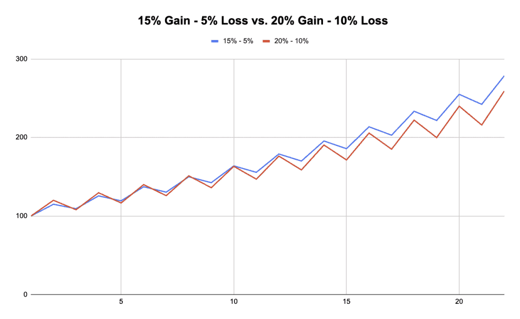
Let’s do this starting from $100 for each.

In this example, we can see that after 22 time periods (where each up and down period is one period), we can see that the value of Bet A (blue line) is $279 while Bet B (red line) is $259.

We can see that Bet B’s greater variance helped it at first, then started lagging over time.

Explanation: Low Volatility Outperforming High Volatility

Volatility Drag

Higher volatility reduces the geometric mean return more than lower volatility does.

This is why leveraged ETFs tend to lag their leverage factor over time.

They only get their leverage factor over the specified timeframe (usually daily), not over multiple periods, and the lag effect gets worse over time.

Consistency

Investments, trades, or returns streams with lower volatility tend to compound more effectively over time, leading to higher long-term returns.

Another Example: – 2% Gain/2% Loss vs. 1% Gain/1% Loss

To compare how quickly you would lose money with an alternating 2% gain/2% loss versus a 1% gain/1% loss, we can calculate the geometric mean return for each scenario and see how they compound over time.

Scenario 1: 2% gain/2% loss alternating

Let’s assume you start with $100.

• After the first period: $100 x 1.02 = $102
• After the second period: $102 x 0.98 = $99.96
• After the third period: $99.96 x 1.02 = $101.96
• After the fourth period: $101.96 x 0.98 = $99.92 …and so on.

The geometric mean return for this scenario is: (0.98 x 1.02)^(1/2) – 1 = -0.00020

So you’ll lose in the long run.

Scenario 2: 1% gain/1% loss alternating

Let’s again assume you start with $100.

• After the first period: $100 x 1.01 = $101
• After the second period: $101 x 0.99 = $99.99
• After the third period: $99.99 x 1.01 = $100.99
• After the fourth period: $100.99 x 0.99 = $99.98 …and so on.

The geometric mean return for this scenario is: (0.99 x 1.01)^(1/2) – 1 = -0.00005

So in the scenario with 1% gain/1% loss alternating, you’ll still lose, but only one-quarter as fast.

This means that in the second scenario with smaller alternating gains/losses, you will lose money at a slower rate compared to the first scenario.

Quantifying It Over Time

To quantify it, if you start with $100 in both scenarios and let them run for 100 periods:

• In scenario 1 (2% gain/loss), your ending value will be: $100 * (1.02 * 0.98)^50 = $98.02
• In scenario 2 (1% gain/loss), your ending value will be: $100 * (1.01 * 0.99)^50 = $99.50

So with the smaller 1% gain/loss scenario, you lose money more slowly.

Why Keeping Drawdowns Low Is Most Important

In trading, limiting drawdowns is extremely important because losses require disproportionately larger gains to recover.

This concept shows the importance of managing volatility and protecting against significant losses.

Here’s why:

The Asymmetry of Losses and Gains

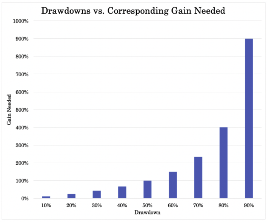
Mathematical Impact of Drawdowns:

• A 10% loss needs an 11% gain to recover.
• A 20% loss requires a 25% gain.
• A 50% loss necessitates a 100% gain.
• As losses deepen, the required recovery gains increase exponentially.

Explanation

1. Compounding Losses:
   • When you experience a loss, the capital base shrinks, meaning subsequent gains are calculated on a smaller amount.
   • For example, if you start with $100 and lose 50%, you have $50. To get back to $100, you need to double your money, which is a 100% gain.
2. Increased Difficulty of Recovery:
   • The deeper the drawdown, the more difficult and time-consuming it becomes to recover.
   • Small losses can be quickly recovered with modest gains, but larger losses require much higher returns, which are harder to achieve consistently.
3. Volatility Drag:
   • High volatility leads to larger drawdowns, which in turn hampers long-term performance due to the asymmetric nature of losses and gains.
   • This “volatility drag” means that even if the average returns (arithmetic mean) are high, the actual compounded returns (geometric mean) will be significantly lower if the investment experiences high drawdowns.

Overall

By limiting drawdowns, traders can protect their capital in a cost-effienct way (more on that below) and be sure that the path to recovery from losses is manageable.

This approach not only stabilizes returns but also maximizes the potential for long-term growth.

This highlights the critical importance of managing volatility and avoiding significant losses in trading strategies.

How to Do This in Practice

To effectively limit drawdowns and manage risk in trading, you can use several strategies:

1. Position Sizing

Risk Per Trade:

• Limit the amount of capital you risk on each trade. A common rule is to risk no more than 1-2% of your total capital on any single security.
• This ensures that even a series of losses won’t significantly deplete your capital.

Adjust Position Size:

• Adjust your position size based on the volatility of the asset. Use smaller positions for more volatile assets to reduce potential drawdowns.
• Techniques like the Kelly Criterion can help as a starting point when it comes to the theory behind determining optimal position sizes.

2. Diversification

Uncorrelated Assets:

• Diversify your portfolio by going into assets or trades that have low or negative correlations with each other.
• Balanced portfolios, even in the context of trading.
• This means that when one asset experiences a drawdown, others may perform well, balancing out the overall portfolio performance.

Multiple Return Streams:

• Create a portfolio with different strategies or asset classes, such as equities, bonds, commodities, and currencies.
• Include strategies like trend-following, mean reversion, and arbitrage to further diversify return streams.

3. Using Options to Cut Off Tail Risk

Protective Puts:

• Purchase protective put options to limit potential losses on your positions.
• This gives you the right to sell your asset at a predetermined price, providing a safety net if the market moves against you.

Collars:

• Implement a collar strategy by buying a put option and selling a call option on the same asset.
• This limits both your downside and upside, effectively creating a range within which your returns will fluctuate.
• The option premium you get from the call helps defray your costs on the protective put option.

Spread Strategies:

• Use spread strategies like vertical spreads, where you buy and sell options at different strike prices but with the same expiration date.
• These strategies can limit potential losses while also reducing the cost of purchasing options.

4. Regular Monitoring and Adjustment

Risk Assessment:

• Monitor your portfolio’s risk profile and make adjustments as needed.
• Use tools like Value at Risk (VaR) and stress testing to assess potential losses under different market conditions.

Rebalancing:

• Regularly rebalance your portfolio to maintain your desired risk level.
• This involves adjusting the weights of different assets to make sure that your portfolio remains diversified and aligned with your risk tolerance.

Conclusion

Understanding the difference between arithmetic and geometric means helps explain why low volatility trades or investments can outperform high volatility ones in the long run.

The geometric mean, accounting for compounding effects, provides a clearer picture of true investment performance.

Through careful position sizing, diversifying across uncorrelated assets/trades/returns streams, using options to manage tail risk, and regularly monitoring and adjusting your portfolio, you can effectively limit drawdowns and protect your capital.

These strategies help stabilize returns and improve the potential for long-term growth.