Kelly Criterion


The Kelly Criterion is a mathematical formula used to determine the optimal size of a series of bets.
Developed by John L. Kelly Jr. in 1956, it has found application in gambling, trading, investing, and risk management.
The criterion aims to maximize the logarithm of wealth.
This offers a strategic edge in scenarios where the probabilities of outcomes are known.
Mathematical Foundation
The Kelly Criterion calculates the proportion of a portfolio to wager, based on the expected return and the odds of the bet.
The formula is expressed as:
Kelly Percentage = (bp – q) / b
Where:
- p is the probability of a winning bet,
- q is the probability of losing (q = 1 − p),
- b is the odds received on the bet (not the probability), defined as the potential winnings divided by the amount wagered.
Example of the Kelly Criterion
Suppose you have a bet where:
- The probability of winning (p) is 0.55 (or 55%).
- The probability of losing (q) is 0.45 (or 45%).
- The odds received on the bet (b) are 1 (even money).
According to the Kelly Criterion, if you have an edge with a 55% chance of winning and even odds, you should wager 10% of your bankroll on each bet to maximize the growth rate of your wealth.
This approach aims to balance the goals of maximizing returns while minimizing the risk of losing the entire bankroll.
This can allow for sustained growth over many bets.
Simulation of Wealth Accumulation Using the Kelly Criterion
Let’s go a step further than what we outlined above and run a simulation of 520 bets (10 year of one bet per week) where you’re getting 55/45 probability (in your favor) on each bet and 1:1 odds.
The chart below illustrates the trajectory of wealth accumulation over time using the Kelly Criterion in this betting scenario.
Here, the initial wealth is set to 100 units, and the individual makes a series of bets over time.
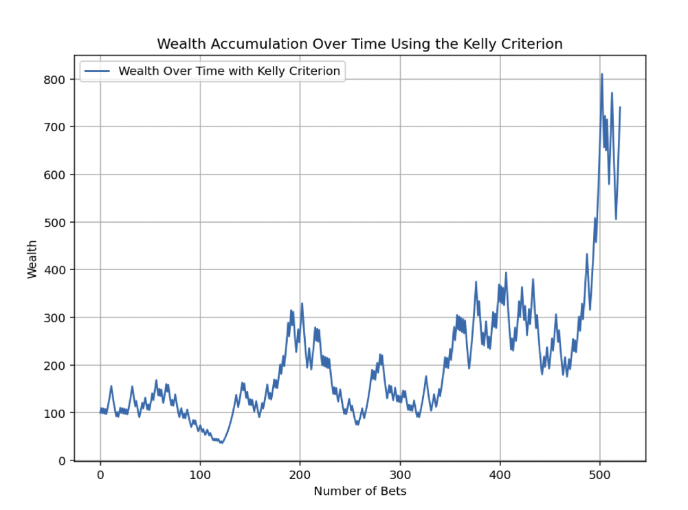
The Good Side to the Kelly Criterion
As seen in the chart, wealth tends to increase over time.
This demonstrates the compounding effect of reinvesting winnings according to the Kelly Criterion.
This simulation shows how using the Kelly Criterion can lead to wealth growth in a probabilistic setting with a positive edge.
The Bad Side to the Kelly Criterion
But it also shows the other side of the Kelly Criterion.
The drawdowns from the high-water mark will be brutal.
We can see between bets 200 and 250, the trader/gambler lost about 70% of his money.
He then promptly doubled again before promptly losing what he made.
He then goes on a big hot streak between bet 460-ish and 500, quadrupling his money.
Upon reaching 800, he then quickly loses over 35%, before a spike back up.
That’s a nice return on one’s money.
But the Kelly Criterion creates a lot of volatility that puts it more in the purview of a risk-seeking gambler than a trader seeking relatively steady gains over time.
Many would psychologically have trouble dealing with this level of volatility and this kind of bankroll management.
More Kelly Criterion Simulations
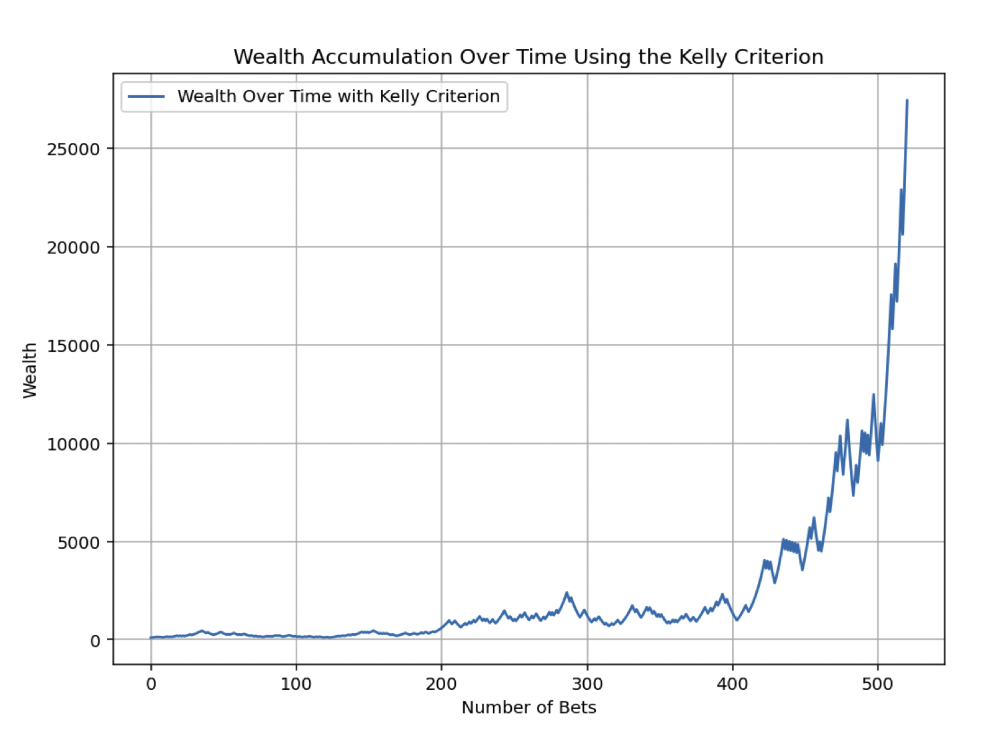
For fun, we ran two more simulations of this.
This one below is great luck, turning 100 into over 25,000 over 520 bets using the Kelly Criterion.
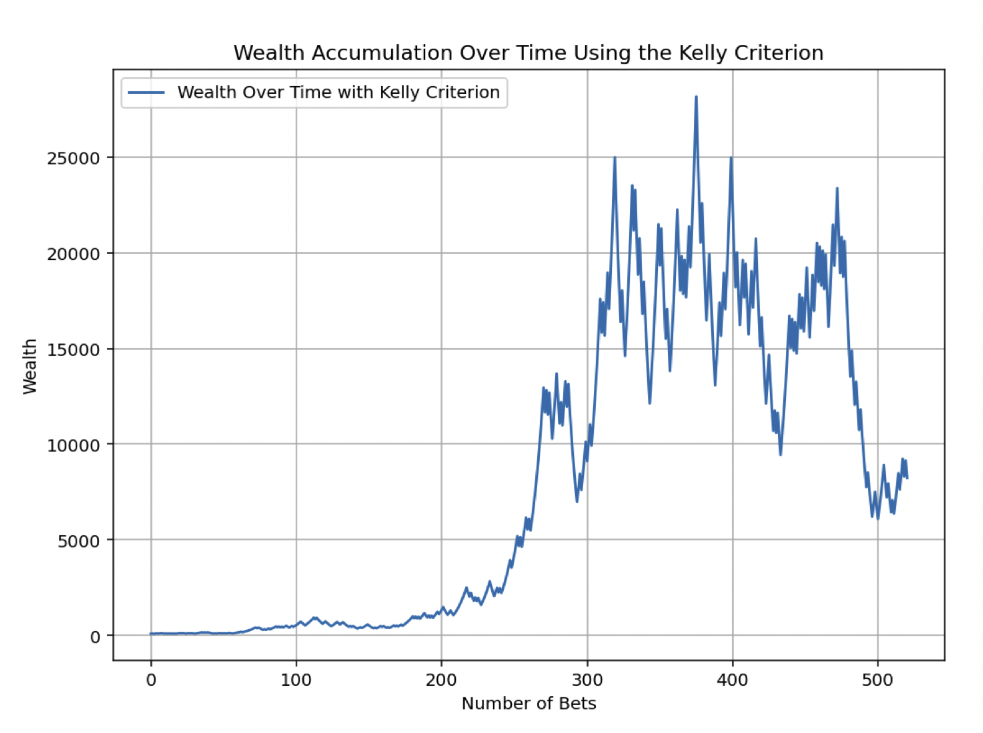
This one has luck early – and faster – but falters down the stretch.
Source Code
If you’d like to try this on your own, this is the Python code:
import numpy as np
import matplotlib.pyplot as plt

# Parameters for the simulation
np.random.seed(42) # for reproducible results
initial_wealth = 100 # initial wealth
n_bets = 520 # number of bets (e.g., 10 years of weekly bets)
b = 1 # odds (b to 1)
p = 0.55 # probability of winning each bet
fraction_kelly = 1 # Fraction of the Kelly Criterion to bet; 1 for full Kelly

# Calculate the Kelly fraction
kelly_fraction = (b * p - (1 - p)) / b

# Simulate the wealth over time using the Kelly Criterion
wealth = [initial_wealth]
for _ in range(n_bets):
bet_size = fraction_kelly * kelly_fraction * wealth[-1]
win = np.random.rand() < p # win or lose the bet
if win:
wealth.append(wealth[-1] + bet_size * b) # update wealth if win
else:
wealth.append(wealth[-1] - bet_size) # update wealth if lose

# Plotting the results
plt.figure(figsize=(12, 6))
plt.plot(wealth, label="Wealth Over Time with Kelly Criterion")
plt.title("Wealth Accumulation Over Time Using the Kelly Criterion")
plt.xlabel("Number of Bets")
plt.ylabel("Wealth")
plt.legend()
plt.grid(True)
plt.show()
If you use this code, be sure to indent as appropriate:

Expected Value of The Kelly Criterion
Let’s run a sim to understand the expected value of this experiment amidst the extreme levels of variance that the Kelly Criterion brings on.
- (probability of winning)
- (probability of losing)
- (the bet pays b to 1; here, it’s even money, so b = 1)
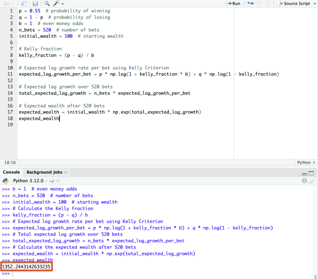
p = 0.55  # probability of winning
q = 1 - p  # probability of losing
b = 1  # even money odds
n_bets = 520  # number of bets
initial_wealth = 100  # starting wealth

# Kelly fraction
kelly_fraction = (p - q) / b

# Expected log growth rate per bet using Kelly Criterion
expected_log_growth_per_bet = p * np.log(1 + kelly_fraction * b) + q * np.log(1 - kelly_fraction)

# Expected log growth over 520 bets
total_expected_log_growth = n_bets * expected_log_growth_per_bet

# Expected wealth after 520 bets
expected_wealth = initial_wealth * np.exp(total_expected_log_growth)
expected_wealth
And we have an expected value of 1,352 (13.5x return on one’s money after 520 bets), showing that we were somewhat unlucky in the first simulation and were lucky in the second and third.
Application in Finance
In finance, the Kelly Criterion is used to think about position sizing and portfolio risks.
It may help as a guiding factor in determining how much capital to allocate to each trade.
By considering the probability of positive returns and the payoff of successful trades, it can guide trade sizing to maximize the growth rate of capital over time.
Nonetheless, the Kelly Criterion isn’t the most appropriate in the context of a sophisticated portfolio where correlation, covariance, and various other factors are at play.
But the general idea of betting more on something when the odds are more in your favor and you’re getting good payoffs or risk premiums holds true – even in the context of those interested in holding balanced portfolios.
Advantages
Long-Term Capital Growth
The Kelly Criterion focuses on maximizing long-term capital growth.
It balances the trade-off between risk and reward.
Risk Management
It inherently considers the risk of ruin and adjusts the bet size accordingly.
It acts as a protective measure against significant losses.
Compounding Interest
Since the strategy is focused on the logarithm of wealth, it implicitly takes advantage of compounding, a key aspect in wealth accumulation.
Limitations
Requirement of Accurate Probabilities
The biggest limitation is the need for precise probabilities of outcomes, which can be challenging to estimate in real-world scenarios.
In the real-world, you rarely know what your odds are.
Volatile Short-Term Performance
The approach can lead to high volatility in the short term, as it often suggests aggressive sizing.
For instance, in our example above, a 55/45 bet with even odds suggests a 10% bet size.
This is quite high and would to a lot of variance.
Sensitivity to Estimation Errors
The formula is sensitive to errors in probability and payoff estimation, potentially leading to suboptimal betting sizes.
Static
Probabilities and payoffs in markets typically fluctuate (and again, are hard to estimate).
Practical Considerations
Fractional Kelly Betting
To mitigate risk, traders often use a fraction of the Kelly Criterion (e.g., half-Kelly).
This reduces potential returns but also decreases risk and volatility.
Diverse Application
Beyond finance, the criterion is used in sports betting, gambling, and other areas where probabilistic outcomes with known odds occur.
Integration with Other Strategies
It is often used in conjunction with other risk management and trading/investment strategies for a more balanced approach.
Conclusion
The Kelly Criterion is used for decision-making in probabilistic environments.
Its ability to maximize wealth over the long term, while considering the risk of large losses, makes it something to at least understand for traders.
Nevertheless, its effectiveness is contingent on the accurate estimation of probabilities and payoffs.
This is a challenge in many practical scenarios.