Risk Parity Strategy Without Bonds – How It Can Be Done


Risk parity is an investment strategy that aims to balance risk across asset classes, rather than allocating more capital to traditionally “safer” investments like bonds.
The goal is to create a portfolio with consistent returns, regardless of market conditions.
It’s also sometimes called balanced beta. It does not generally involve any tactical trading outside rebalancing to remain portfolio allocations.
The typical risk parity portfolio includes a mix of stocks, commodities, and other asset classes.
But what if you want to pursue a risk parity strategy without including bonds? Is it possible?
Key Takeaways – Risk Parity Strategy Without Bonds
- Risk parity balances risk across assets, not just capital weights.
- The goal is steadier results across different macro environments (rising/falling growth/inflation – i.e., four quadrants).
- Traditional risk parity uses bonds because they’re typically less volatile than stocks and can offset equity drawdowns during growth shocks (much less reliably during inflation shocks).
- A bond-free version is possible when nominal bonds offer poor real yields or weak risk compensation.
- Main options = increase allocations to non bond diversifiers and add return streams with lower volatility characteristics.
- Key non-bond building blocks = equities, commodities, gold, real assets, CTA strategies, and inflation-linked bonds like TIPS.
- Without bonds, add crisis alpha strategies like managed futures or selective long volatility to replace missing convexity.
- Lower the volatility of your equity portion with defensive sectors (utilities, consumer staples, healthcare) or a min-vol fund so risk is easier to balance. Remember they are still stocks and can fall if growth or rates incur a shock.
- Risk parity needs leverage. Get it cheaply through index futures, capital-efficient ETFs like GDE, return-stacked funds, or lower-cost margin at a broker like Interactive Brokers. Avoid daily-reset leveraged ETFs for long holds.
- Goal is ultimately survival and compounding, not maximum upside in equity bull markets.
The short answer
The short answer is yes; it’s possible to pursue a risk parity strategy without including bonds in your portfolio, or at least the type of bonds that offer bad returns relative to inflation and overall risk.
Or those that correlate too much to other return streams in your portfolio because they take on too much credit risk to get sufficient yield, or too much duration risk and therefore are at risk of losing value due to higher interest rates (also a drag on stocks, all else equal).
There are a few different ways to do this, which we’ll outline below.
Allocate to other asset classes
One way to go about pursuing a bond-free risk parity strategy is to simply allocate more capital to the other asset classes in your portfolio.
This means you would have a higher percentage of stocks and commodities, for example. Or other things that can serve as stores of value.
Focus on investments with high returns and lower volatility
Another way to pursue a bond-free risk parity strategy is to focus on investments that offer high returns and perhaps lower volatility.
This could include things like cash-flowing real estate or private equity, though both are still subject to the same economic forces as other forms of equity even if their returns aren’t marked to market. Risk simply doesn’t go away even when an asset is private and its price is “hidden.”
Ultimately, there is no one right way to pursue a bond-free risk parity strategy. It will depend on your specific goals and investment objectives.
But if you’re looking for ways to balance risk in your portfolio without including bonds, these are two options to consider.
And even if bonds are bad investments from a real returns perspective, some might even argue including some smaller amount of nominal rate bonds for their diversification value.
The problem with bonds today
Bonds are favored by many market participants because they’re generally safe:
- They have a fixed payout.
- They have a fixed maturity, making them less volatile than stocks.
- They’re senior to equity holders in the case of a company, so bondholders get paid first in the case something happens to the company.
But when looking at bond yields in your domestic currency, you have to look at your real yield; that is, your yield after adjusting for inflation.
If a bond yields 5 percent but inflation is 5 percent, you haven’t made anything in real terms; i.e., you haven’t gained purchasing power.
When looking at bond yields in foreign currency, what’s important is the yield relative to the movement in the exchange rate between the foreign currency and the one you make your payments in.
For example, if a bond yields 8 percent in a foreign currency, but that currency falls by 8 percent against your own currency, you made nothing in nominal terms.
Bonds have been mostly poor investments on a yield basis since the 2008 financial crisis, already a long time ago.
Though bond yields have crept up since 2020, inflation also increased and eroded the benefits of higher nominal yields.
Below is a chart of the US 10-year yield on an inflation-adjusted basis.
Market Yield on US Treasury Securities at 10-Year Constant Maturity, Quoted on an Investment Basis, Inflation-Indexed
(Source: Board of Governors of the Federal Reserve System (US))
Before getting 2-3 percent real returns on a 10-year bond was considered normal.
After 2008, anywhere from minus-1 to plus-1 percent has been the new norm.
With lower yields, means less return for each unit of volatility/risk.
This is pushing all kinds of private investors into other asset classes, not only those in risk parity.
How risk parity normally uses bonds
Stocks are about 3x as volatile as mid-duration government bonds.
This is because the cash flows of stocks are theoretically perpetual while those of bonds are fixed (the bond matures on a certain date).
And government bonds are backed by the government, which makes their cash flows generally more secure. In a reserve-currency country, they will always pay their bills in nominal terms.
But under approaches like a 60/40 portfolio, because stocks are more volatile than bonds, the risk ends up concentrated nearly 90 percent in stocks rather than the ostensible balance of weighting them by close to equal amounts of capital.
Risk parity aims to fix this by leveraging the fixed income side so that the risk of the bonds matches that of stocks and other assets in the portfolio.
This is normally done by borrowing cash to buy more bonds (easier to do when the yield curve is steep) or by using leverage-like techniques such as by buying futures to replicate higher bond exposure at a small collateral obligation. Or perhaps even through options.
But when the return on bonds weakens, the case for a higher allocation toward other assets grows.
The 4 Quadrants
Many balanced beta approaches think of portfolios as having assets that can perform no matter what the big two macro forces (growth and inflation) are doing relative to discounted expectations.
That gives four quadrants – rising/falling growth and inflation – with the idea of putting 25% of your risk into each.
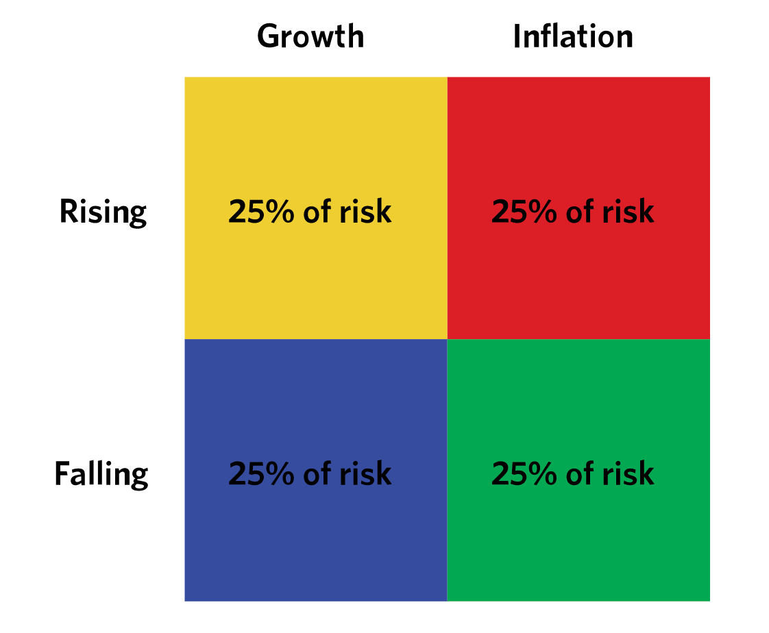
Spreading risk evenly is done to avoid assuming the market has a systematic bias toward over- or under-discounting future growth or inflation outcomes.
How do individual asset classes fit in?
One interpretation is shown below. This is simply illustrative. It’s not necessarily indicative of any actual historical or current implementation of the strategy.
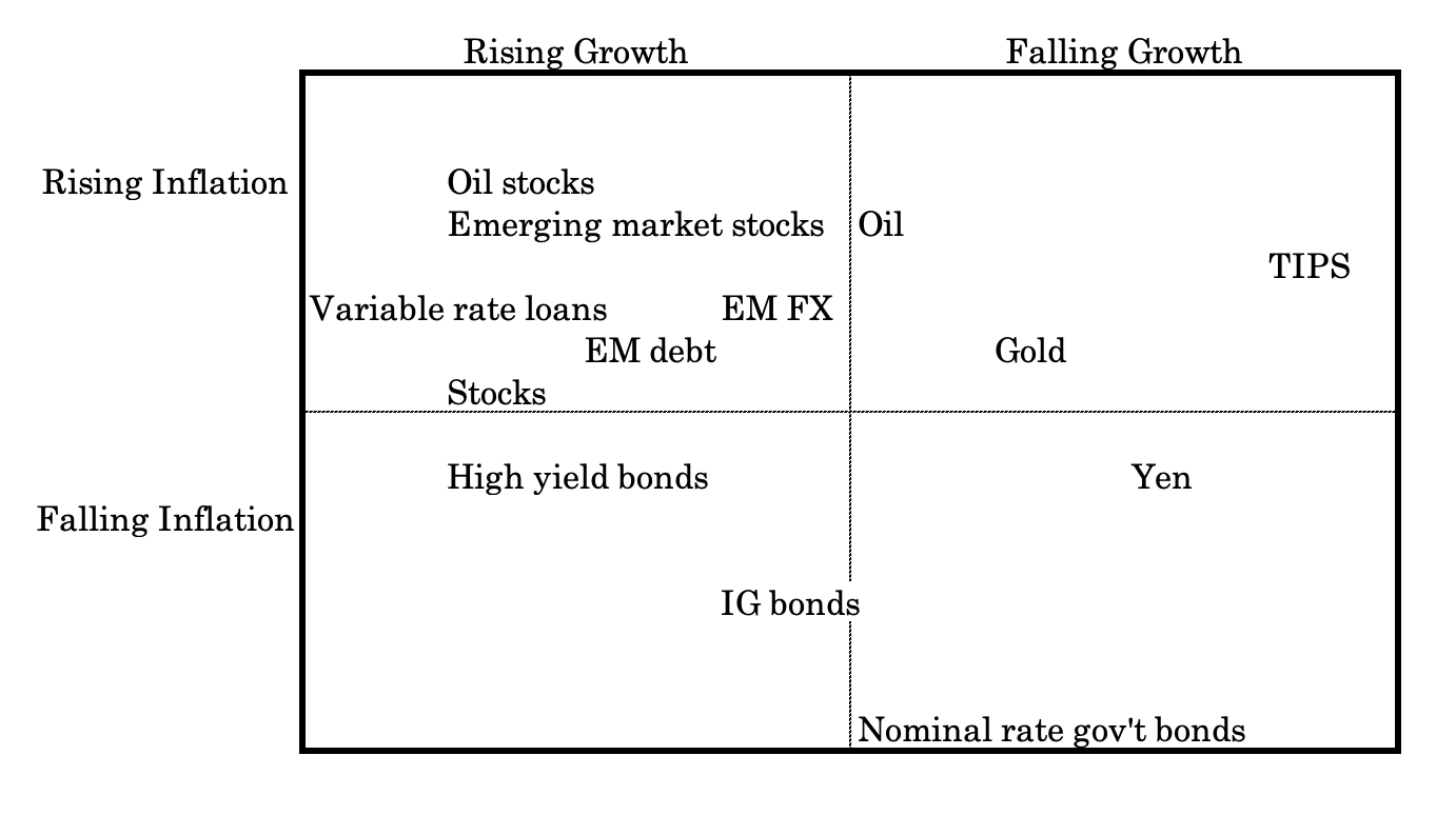
Also note that no specific asset class is necessarily a perfect rising/falling growth/inflation asset.
Some can be in the same bucket but on a different part of the spectrum.
Stocks and corporate bonds would be an example. Stocks react more favorably to higher discounted growth and corporate bonds are less growth-sensitive than equities.
Investment-grade (IG) corporate bonds are a falling inflation asset. But they’re neither particularly biased heavily toward higher or lower growth. Higher growth benefits corporations and their bonds, but the demand for safety and liquidity increases as markets fall. Safe corporate bonds are often one avenue where this capital flows.
For example, when the stock market (i.e., S&P 500) fell 37% in 2008, safe corporate bonds actually rose slightly.
For example, oil is clearly a rising inflation asset, in general, and is sometimes the cause of inflation its impact on growth is not as clear. For oil-exporting countries, its impact on growth is positive; for oil-importing countries, its impact on growth is negative, all else equal.
Cheap ways to add leverage when you skip bonds
Risk parity needs leverage. That is the part people skip over. The whole method is to size each asset so it contributes a similar amount of risk, then scale the package up to the risk level you actually want.
When you drop nominal bonds, you lose the asset that was easiest and cheapest to lever, because deep Treasury futures markets and a steep yield curve made borrowing against bonds simple.
So you have to get your leverage somewhere else, and you want it cheap. Every percentage point of borrowing cost comes straight out of your return.
Here are the main ways to do it, roughly from cheapest to most convenient.
Index and commodity futures
This is the cheapest structural leverage available to most investors.
An E-mini S&P 500 contract (ticker ES) controls about $50 times the index, and the Micro E-mini (MES) controls one-tenth of that.
Gold has the same setup: the full contract (GC) covers 100 ounces, and the micro (MGC) covers 10.
You post a bit in margin (often around 10%) and get the full notional position. The financing cost baked into a futures price sits close to the risk-free rate, which is far below what a retail margin loan charges.
You roll the contract each quarter. In the US, futures also get favorable tax treatment under Section 1256, where gains are taxed 60 percent long-term and 40 percent short-term regardless of holding period.
The downsides are lumpy contract sizes and daily mark-to-market, so you have to manage margin actively.
Capital-efficient ETFs
These pack leverage into a single ticker. The clearest fit for a bond-free portfolio is the WisdomTree Efficient Gold Plus Equity Strategy Fund (GDE).
For every $1 you invest, it delivers roughly $0.90 of S&P 500 exposure and $0.90 of gold exposure through futures, all for about a 0.20 percent expense ratio.
GDE has a shorter history, going back to just 2022:
Asset Correlations
| Name | Ticker | SPY | GDE | Annualized Return | Daily Standard Deviation | Monthly Standard Deviation | Annualized Standard Deviation |
|---|---|---|---|---|---|---|---|
| State Street SPDR S&P 500 ETF | SPY | 1.00 | 0.75 | 14.70% | 1.09% | 4.70% | 16.27% |
| WisdomTree Efcnt Gld Pls Eq Stgy ETF | GDE | 0.75 | 1.00 | 29.81% | 1.65% | 6.25% | 21.64% |
| Asset correlations for time period 04/01/2022 – 05/31/2026 based on monthly returns | |||||||
So you get a bond-free risk parity building block you can buy in a brokerage account. WisdomTree’s NTSX does the same thing with stocks and Treasuries (90 percent S&P 500 plus 60 percent Treasury futures) if you do want some bond duration in the mix.
NTSX goes back to 2018:
Asset Correlations
| Name | Ticker | SPY | NTSX | Annualized Return | Daily Standard Deviation | Monthly Standard Deviation | Annualized Standard Deviation |
|---|---|---|---|---|---|---|---|
| State Street SPDR S&P 500 ETF | SPY | 1.00 | 0.98 | 14.93% | 1.23% | 4.91% | 17.00% |
| WisdomTree U.S. Efficient Core Fund | NTSX | 0.98 | 1.00 | 12.82% | 1.16% | 4.75% | 16.47% |
| Asset correlations for time period 09/01/2018 – 05/31/2026 based on monthly returns | |||||||
Though NTSX is slightly leveraged over SPY, the diversification brings down the average volatility slightly.
Return-stacked ETFs
The Return Stacked family layers a second return stream on top of a full equity or bond position using internal leverage.
RSST gives you $1 of US large-cap stocks plus $1 of a managed futures strategy for every $1 invested.
Asset Correlations
| Name | Ticker | SPY | RSST | Annualized Return | Daily Standard Deviation | Monthly Standard Deviation | Annualized Standard Deviation |
|---|---|---|---|---|---|---|---|
| State Street SPDR S&P 500 ETF | SPY | 1.00 | 0.80 | 25.35% | 0.98% | 3.74% | 12.95% |
| Return Stacked US Stocks&Mgd Futs ETF | RSST | 0.80 | 1.00 | 23.64% | 1.53% | 5.19% | 17.99% |
| Asset correlations for time period 10/01/2023 – 05/31/2026 based on monthly returns | |||||||
RSSY pairs $1 of stocks with $1 of a futures-yield (carry) strategy.
Asset Correlations
| Name | Ticker | SPY | RSSY | Annualized Return | Daily Standard Deviation | Monthly Standard Deviation | Annualized Standard Deviation |
|---|---|---|---|---|---|---|---|
| State Street SPDR S&P 500 ETF | SPY | 1.00 | 0.68 | 21.26% | 1.05% | 3.60% | 12.47% |
| Return Stacked US Stk&Futs Yld ETF | RSSY | 0.68 | 1.00 | 13.50% | 1.16% | 5.01% | 17.37% |
| Asset correlations for time period 06/01/2024 – 05/31/2026 based on monthly returns | |||||||
RSSX pairs $1 of stocks with $1 of a gold-and-bitcoin portion.
Asset Correlations
| Name | Ticker | SPY | RSSX | Return | Daily Standard Deviation | Monthly Standard Deviation | Annualized Standard Deviation |
|---|---|---|---|---|---|---|---|
| State Street SPDR S&P 500 ETF | SPY | 1.00 | 0.83 | 29.82% | 0.75% | 3.79% | 13.14% |
| Return Stacked US Stks&Gold/BitcoinETF | RSSX | 0.83 | 1.00 | 39.03% | 2.00% | 7.08% | 24.54% |
| Asset correlations for time period 06/01/2025 – 05/31/2026 based on monthly returns | |||||||
For a bond-free book, a fund like RSST lets you hold your full equity exposure and stack a trend-following crisis-alpha portion on top without carving out separate capital for it.
Expense ratios run around 0.95 to 1.05%
Margin loans
This is the route most retail investors actually use, and the broker matters enormously.
At Interactive Brokers Pro, a margin loan costs the firm’s benchmark rate, which tracks the fed funds rate, plus a spread of roughly 0.5 to 1.5 percent depending on how much you borrow, with the spread shrinking as the loan grows.
There is a 0.75 percent minimum floor. Many traditional brokers charge 8 to 10 percent on comparable balances, so Interactive Brokers can run less than half the cost.
If you qualify for portfolio margin (generally accounts above roughly $110,000), the broker sets your borrowing requirement based on stress-tested scenarios across your whole portfolio rather than crude per-position rules, so a diversified risk parity book gets more room than standard Reg-T margin allows.
Box spreads
For larger accounts, this is often the cheapest borrowing of all. A box spread is a package of SPX options that locks in a fixed loan at a known rate.
Why SPX? Because they’re European-style and so there’s no early assignment risk.
Investors use them to borrow at close to Treasury-bill yields, frequently within a few tenths of a percent of where Treasuries trade.
They require options approval and some care to set up correctly, but for sizable balances they can undercut even Interactive Brokers margin.
One warning that applies to all of this. Leverage cuts both ways, and not all leverage is equal. Avoid daily-reset leveraged ETFs like UPRO (3x) or SSO (2x) for holds beyond one day.
Their daily rebalancing creates volatility drag, so in a choppy, sideways market they bleed value even when the index finishes flat.
For a long-term risk parity position, structural leverage holds its exposure without that decay, whether you use futures, a capital-efficient ETF, a return-stacked fund, or a plain margin loan.
And size it so a sharp selloff won’t trigger a forced liquidation at the worst possible moment.
A sensible rule for most = keep total notional modest, hold a cash buffer, and stress-test/pre-mortum what a 30 to 40 percent equity drop would do to your margin before you ever need to know.
Other asset classes outside bonds
Without nominal rate bonds you have other asset classes including:
Inflation-indexed bonds (ILBs)
Inflation-indexed bonds, also known as linkers or inflation-linked bonds, adjust the face value of the bond according to changes in a consumer price index (CPI).
It’s important to note that inflation-linked bonds carry interest rate risk just like nominal rate bonds.
They are not pure inflation investments that simply give you the price level.
For those looking for more of a pure investment, i.e., does well when inflation rises faster than discounted expectations, they would be looking at an inflation swap or CPI swap.
This is a type of OTC derivative available to institutional investors.
For those who don’t have access to inflation or CPI swaps, one can go long an ILB and short the equivalent tenor nominal rate bond.
For example, one might go long a 10-year TIPS bond and short a 10-year US Treasury nominal rate bond.
If discounted inflation expectations rise, the trader or investor would benefit similar to an inflation swap.
Equities
Equities (stocks) are one of the most common asset classes.
There are different types of stocks, including:
- Growth stocks = Companies that are expected to grow at a faster rate than the markets they compete in
- Value stocks = Companies that may be undervalued by the market and offer potential for capital appreciation
- Dividend stocks = Companies that pay out regular dividends to shareholders
Lower-volatility equities: utilities, staples, and healthcare
One way to make risk balancing easier without bonds is to lower the volatility of the equity part itself.
Some equity sectors carry less risk than the broad market because their earnings hold up regardless of where you are in the economic cycle.
When your stocks swing less, the gap between equity risk and the risk of your other assets shrinks, so you need less offset to balance the book and often less leverage overall.
Three sectors do most of this work.
Utilities
Regulated electric, gas, and water companies earn returns set by public commissions, so their cash flows are steady and predictable.
The sector ETF XLU typically runs a beta around 0.4 to 0.6 against the S&P 500, with dividend yields often near 3 percent. VPU is another popular ETF with around double the holdings of XLU.
Holdings include NextEra Energy (NEE), Duke Energy (DUK), and Southern Company (SO).
The catch is that utilities carry heavy debt and pay high dividends, so they trade like bond substitutes.
When interest rates jump, utilities tend to fall alongside both stocks and bonds, which is exactly the scenario that punished every “safe” asset in 2022. So they cut your growth-shock risk but add rate-shock risk.
Consumer staples
People buy toothpaste, soap, and groceries in any economy, so staples earnings are inelastic.
XLP holds Procter & Gamble (PG), Coca-Cola (KO), Costco (COST), Walmart (WMT), and Colgate-Palmolive (CL).
Beta typically lands around 0.5 to 0.6. In the 2008 crash, staples fell far less than the S&P 500 and recovered faster. The trade-off is slow growth, and at times rich valuations when nervous investors crowd in for safety and bid the sector up and future returns down.
Healthcare
Demand for medicine and care does not wait for the cycle, and an aging population adds a long-run tailwind.
XLV holds UnitedHealth (UNH), Johnson & Johnson (JNJ), Merck (MRK), AbbVie (ABBV), and Eli Lilly (LLY).
Beta here is generally around around 0.6 to 0.7, a notch higher than utilities or staples.
The main risks are policy (drug pricing rules, reimbursement changes) and patent cliffs at individual companies, which is one reason a diversified sector ETF beats betting on a single name.
How much worse are their returns?
We can see from the graph below that utilities generally underperform the market by about 1% (with roughly the same volatility), consumer staples typically underperform by about 2% (with less risk), and healthcare trails by about 0-1% with slightly less risk.
Asset Correlations
| Name | Ticker | SPY | XLU | XLP | XLV | Annualized Return | Daily Standard Deviation | Monthly Standard Deviation | Annualized Standard Deviation |
|---|---|---|---|---|---|---|---|---|---|
| State Street SPDR S&P 500 ETF | SPY | 1.00 | 0.46 | 0.61 | 0.76 | 8.71% | 1.21% | 4.37% | 15.12% |
| State StreetUtilSelSectSPDRETF | XLU | 0.46 | 1.00 | 0.58 | 0.42 | 7.66% | 1.21% | 4.39% | 15.20% |
| State StreetCnsmrStpSelSectSPDRETF | XLP | 0.61 | 0.58 | 1.00 | 0.58 | 6.61% | 0.96% | 3.60% | 12.48% |
| State StreetHlthCrSelSectSPDRETF | XLV | 0.76 | 0.42 | 0.58 | 1.00 | 8.16% | 1.12% | 4.10% | 14.19% |
| Asset correlations for time period 01/01/1999 – 05/31/2026 based on monthly returns | |||||||||
If you combined these three into one portfolio:
| Ticker | Name | Allocation |
|---|---|---|
| XLU | State StreetUtilSelSectSPDRETF | 34.00% |
| XLP | State StreetCnsmrStpSelSectSPDRETF | 33.00% |
| XLV | State StreetHlthCrSelSectSPDRETF | 33.00% |
10 years of backtesting shows lower return at around 20% less volatility but still a 72% correlation to the index.
Performance Summary
| Metric | Portfolio 1 | Portfolio 2 | Vanguard 500 Index Investor |
|---|---|---|---|
| Start Balance | $10,000 | $10,000 | $10,000 |
| End Balance | $39,225 | $23,623 | $39,073 |
| Annualized Return (CAGR) | 15.62% | 9.56% | 15.57% |
| Standard Deviation | 15.71% | 12.36% | 15.74% |
| Best Year | 31.22% | 24.61% | 31.33% |
| Worst Year | -18.17% | -2.03% | -18.23% |
| Maximum Drawdown | -23.93% | -14.28% | -23.95% |
| Sharpe Ratio | 0.85 | 0.60 | 0.85 |
| Sortino Ratio | 1.34 | 0.93 | 1.33 |
| Active Return | 0.05% | -6.01% | N/A |
| Tracking Error | 0.30% | 10.93% | N/A |
| Information Ratio | 0.16 | -0.55 | N/A |
| Benchmark Correlation | 1.00 | 0.72 | N/A |
Low-volatility factor funds
Rather than pick sectors, you can buy a rules-based fund that selects the least volatile stocks across the whole market.
The iShares MSCI USA Min Vol Factor ETF (USMV) and the Invesco S&P 500 Low Volatility ETF (SPLV) both aim for smaller drawdowns and tend to run betas around 0.7.
They naturally tilt toward staples, utilities, and healthcare but spread the bet wider across the market.
In the 2020 COVID crash and the 2022 selloff, both gave up less than the broad index, though they also lagged in strong bull runs.
Over USMV’s history, the S&P 500 has still outperformed in risk-adjusted terms (and naturally, in absolute terms).
Asset Correlations
| Name | Ticker | SPY | USMV | Annualized Return | Daily Standard Deviation | Monthly Standard Deviation | Annualized Standard Deviation |
|---|---|---|---|---|---|---|---|
| State Street SPDR S&P 500 ETF | SPY | 1.00 | 0.86 | 15.12% | 1.05% | 4.04% | 13.99% |
| iShares MSCI USA Min Vol Factor ETF | USMV | 0.86 | 1.00 | 11.51% | 0.85% | 3.23% | 11.18% |
| Asset correlations for time period 11/01/2011 – 05/31/2026 based on monthly returns | |||||||
The same is true with SPLV:
Asset Correlations
| Name | Ticker | SPY | SPLV | Annualized Return | Daily Standard Deviation | Monthly Standard Deviation | Annualized Standard Deviation |
|---|---|---|---|---|---|---|---|
| State Street SPDR S&P 500 ETF | SPY | 1.00 | 0.75 | 14.20% | 1.08% | 4.14% | 14.33% |
| Invesco S&P 500 Low Volatility ETF | SPLV | 0.75 | 1.00 | 9.74% | 0.91% | 3.37% | 11.68% |
| Asset correlations for time period 06/01/2011 – 05/31/2026 based on monthly returns | |||||||
How specifically do these min-vol funds help if they also lag in risk-adjusted terms?
So, the broad S&P 500 runs about 14 to 17 percent annual volatility. A blend tilted toward defensive sectors, or a min-vol fund, might run closer to 11 to 13 percent.
That smaller equity swing means your gold, commodity, TIPS, and managed-futures sleeves don’t have to work as hard to balance the portfolio’s risk.
You give up some upside, because lower beta means you capture less of a roaring bull market. For a strategy built around steady compounding rather than maximum upside, that is an acceptable trade.
Also, defensive equities are still equities. They lost money in 2008 and 2020, just less of it.
They don’t give you the negative-correlation or low-correlation offset that bonds or managed futures can provide in a growth shock.
And the most rate-sensitive of them, utilities in particular, can move down with bonds during an inflation shock, which is the very problem that pushed you away from bonds in the first place.
Treat them as a lower-octane version of your equity exposure. They’re still more equity-like than a genuine bond replacement.
Commodities
Commodities are natural resources that can be bought and sold.
They include things like precious metals (gold, silver, platinum), energy (oil, nat gas), agricultural products (wheat, corn, soybeans), and base metals (copper, zinc).
Commodities have low correlations with both stocks and bonds because they tend to do well in an inflationary environment (and can even be the cause of inflation itself to a partial or full degree), so they can act as a good diversifier.
And because commodities are priced in dollars (or other currencies), their prices tend to go up when the dollar falls.
This provides some protection against currency debasement, which is often a byproduct of inflation.
So, in some ways, inflation can be thought of as alternative currencies, assets with real value, and follow the “inverse money” concept in that their values are partially attributed to the value of the money used to buy them.
Real estate
Real estate is another asset class that can offer quality returns.
There are different types of real estate investments, including:
- Residential real estate – This could include things like single-family homes, condominiums, and apartments. This excludes personal residences, as the nominal appreciation typically doesn’t offset inflation and the negative carry and transaction costs.
- Commercial real estate – This could include office buildings, retail space, warehouses, and storage units.
- Industrial real estate – This could include factories, manufacturing plants, and distribution centers.
Most real estate is illiquid, which shouldn’t be confused for safe just because you can’t see the price.
Private equity and private businesses
Private equity is a type of investment that’s not traded on public markets.
It typically involves investing in companies that are not publicly traded, or that are going through a major transition such as a merger or acquisition.
Private equity can offer high returns, but can also be a higher-risk investment, depending on the exact nature of what’s being done.
Private businesses are another type of investment that can offer high returns.
These are businesses that are not publicly traded, and they can include anything from small businesses to large companies.
Investing in private businesses can be a risky investment, but it can also offer the potential for high returns.
When it comes to institutional private equity, there are two types of funds: buyout and growth.
With a buyout fund, the focus is on acquiring a controlling interest in a company and then improving its operations to increase the value of the business.
With a growth fund, the focus is on investing in companies that are expected to experience high levels of growth.
Growth funds can be more risky than buyout funds, but they also have the potential for higher returns.
And growth is also closer on the spectrum toward venture capital.
Most small business opportunities provide the opportunity for higher returns than traditional investments in the stock market.
Other bonds that are “good”
If there are bonds that are yielding less than (or well less than) the rate of inflation, you can avoid those by looking for better ones.
These can include:
- Inflation-linked bonds (aforementioned)
- Foreign currency bonds (they can also provide some level of diversification)
- Corporate bonds
That way you can have access to different countries and different currencies (an important part of the overall diversification process) without having to put all your bond allocation in a certain country (e.g., US) or from a certain issuer (e.g., federal government).
You can also look at different maturities, since bonds with longer terms will generally have higher yields than bonds with shorter terms.
However, you need to be careful with long-term bonds, because if interest rates rise you could end up losing money on your investment on a mark-to-market basis.
Moreover, with corporate bonds, you have to keep a keen eye on credit risk. Bonds with high yields often price a higher-than-comfortable risk of bankruptcy.
Crisis Alpha and Tail Strategies
Crisis alpha and tail behavior return streams, e.g., CTA/managed futures strategies, are beneficial for improving a risk parity framework that excludes bonds.
This is because they address the primary structural weakness of bondless portfolios: the loss of natural convexity and deflation protection.
Traditional risk parity relies on long-duration bonds, or duration-matched to the rest of the portfolio, to provide both volatility ballast and crisis offset.
When bonds are removed, whether its due to inflation risk, low/zero/negative real yields, or policy skepticism, the portfolio becomes more structurally exposed to left-tail events.
Crisis alpha backtests are designed to replace that missing convexity.
Dynamic Convexity
First, trend-following overlays during equity drawdowns introduce dynamic convexity that doesn’t depend on duration.
Time-series momentum strategies typically reduce or short equity exposure as volatility rises and prices trend downward.
Backtesting this overlay shows that it converts part of the equity risk from linear to asymmetric.
Losses are capped earlier in sustained drawdowns. This improves drawdown depth and recovery time.
This improves risk parity by stabilizing risk contributions during crises rather than letting equity dominate total portfolio risk.
Less Dependence on Static Diversification
Second, long volatility strategies versus traditional hedges address the failure mode of static diversification.
In bondless portfolios, correlations are more likely to converge toward one during stress.
Long volatility exposures, such as variance risk premia (i.e., volatility risk premium) or systematic volatility buying, explicitly benefit from that correlation spike.
Backtests show that while these strategies often have negative carry in calm periods, they materially improve left-tail outcomes.
The result is a portfolio that accepts small ongoing costs in exchange for crisis convexity, which is what bonds historically provided.
But they don’t necessarily do that all the time, especially when inflation volatility is the main macro driver of asset returns.
Related: List of Risk Premia
Survival = Top Priority
The core question is survival. A bondless risk parity portfolio that incorporates crisis alpha mechanisms is no longer optimizing Sharpe under stable conditions.
It’s designed to withstand equity shakedowns, regime breaks, preserve capital, and maintain optionality when macro assumptions fail.
Stack crisis alpha on top of equities with return stacking
The hard part of adding managed futures or long volatility to a portfolio is funding it.
Every dollar you put into a CTA is a dollar not in stocks, so in a calm bull market the diversifier drags on returns and you feel the cost.
That cost is the main reason traders abandon these strategies before they pay off over a full cycle or multi-cycle time horizon. Return stacking solves the funding problem.
Instead of carving capital out of equities, you hold full equity exposure and layer the crisis-alpha part on top using internal leverage.
A fund like RSST gives you $1 of US large-cap stocks and $1 of a managed-futures strategy for every $1 invested. So a 20 percent slice of RSST adds 20 percent managed-futures exposure while keeping the 20 percent of equity it replaced.
You hold your equity beta and get the trend-following convexity that tends to pay off during sustained selloffs, in the same dollar.
RSSY does the same with a carry (futures-yield) strategy stacked on stocks, and RSSX stacks a gold-and-bitcoin overlay on stocks for investors who want alternative asset diversification without giving up equity.
You can build the same thing yourself with futures, but the wrapper handles the rolling, margin, and rebalancing for you.
The cost is the expense ratio (roughly 0.95 to 1.05 percent for these funds) and the same leverage risks covered above: the stacked exposure increases both gains and losses, and the diversifier can still lose money in a calm market.
But the structure is a big part of what you pay for. You stop choosing between equity upside and crisis protection and hold both at once, which is the exact problem a bond-free risk parity portfolio is built to solve.
Example of a risk parity portfolio without bonds (or bonds that aren’t terrible)
Above, we established that the main problem with bonds is their low yields relative to inflation in most countries.
This is especially true in reserve-currency countries, such as bonds denominated in dollars, euros, yen, and other reserve currencies.
Inflation-indexed bonds, foreign bonds, and higher-yielding corporate bonds can be a part of your portfolio.
If you go too heavily in any asset class, your portfolio will have a tendency to behave well in certain environments and poorly in others.
For example, many retirees are afraid of owning stocks because they don’t want the volatility.
But if they concentrate too heavily in cash and safer bonds, their portfolio will also have environmental bias.
Their portfolio might suffer when growth is above expectation and inflation runs higher. They could compensate for this risk by buying something different from what they already have (such as stocks or commodities) to help offset it.
Here is an example portfolio:
| Asset Class | Allocation |
|---|---|
| Global Stock Market | 25.00% |
| Gold | 12.00% |
| Commodities | 8.00% |
| TIPS | 35.00% |
| Long-Term Corporate Bonds | 10.00% |
| Total US Bond Market | 5.00% |
| Global Bonds (Unhedged) | 5.00% |
The portfolio returns below assume a starting amount of $100,000 and fixed $1,000 contributions per month, with those contributions inflation-adjusted.
The compounded annual gross returns (CAGR) reflect this below.
The time-weighted rate of return (TWRR) is another measure of the compound rate of growth in a portfolio. The TWRR helps eliminates the effects on growth rates created by inflows and outflows of money that would distort standard return numbers.
The money-weighted rate of return (MWRR) refers to the discount rate that equates a project’s present value cash flows to its initial investment. The MWRR is also sometimes called the internal rate of return (IRR).
These portfolio returns are from 2007 forward, given the data for the commodities asset class only went back to that year.
| Portfolio | Initial Balance | Final Balance | CAGR | TWRR | MWRR | Stdev | Best Year | Worst Year | Max. Drawdown | Sharpe Ratio | Sortino Ratio | Market Correlation |
|---|---|---|---|---|---|---|---|---|---|---|---|---|
| Portfolio 1 | $100,000 | $550,412 | 11.63% | 5.37% | 5.28% | 7.68% | 17.05% | -13.27% | -21.57% (-17.55%) | 0.62 | 0.88 | 0.77 |
The charts below show portfolio returns in both nominal (top) and real (bottom) terms:
Annual returns by year:
Drawdowns:
More statistics and charts about this portfolio are included in the appendix at the bottom of this article.
Size your risk without bonds: inverse-vol and volatility targeting
Risk parity isn’t owning a bit of everything. It’s sizing them so each contributes a similar amount of risk, then scaling the whole package to the risk level you want. Two methods do most of the work, and you can apply both without a single bond.
Inverse-volatility weighting
Weight each asset by the inverse of its volatility, so the calmer assets get more capital and the wilder ones get less.
Take the four assets in the portfolio that follows: the S&P 500 part runs about 15 percent volatility, gold about 20 percent, managed futures about 11 percent, and TIPS about 6 percent.
Pure inverse-vol weighting would tilt heavily toward TIPS and managed futures and trim the equity and gold weight, because $1 in stocks carries almost three times the risk of $1 in TIPS.
This is a rough first cut that gets you most of the way to balanced risk without any optimization.
Account for correlation
Inverse-vol ignores how assets move together.
Two assets at 15 percent volatility that move in lockstep contribute far more combined risk than two that move independently.
True risk parity uses the covariance matrix to equalize each asset’s marginal contribution to total portfolio risk.
A managed-futures sleeve earns a larger weight than its volatility alone would suggest, because its negative correlation to equities, around -0.18 in the data below, reduces total risk rather than adding to it.
Volatility targeting
Once weights are set, scale total exposure to hit a target portfolio volatility, say 10 percent.
When realized volatility is low, you lever up to reach the target. When markets get wild and volatility spikes, you cut exposure to stay at the target.
This is how some funds run risk parity, and it’s the main reason their drawdowns in a crisis are smaller than a static allocation: the book automatically de-risks as volatility climbs.
The trade-off is turnover, and in a fast V-shaped recovery, the risk of cutting exposure right before a rebound.
The practical version:
- pick weights using inverse-vol as a starting point
- adjust toward the assets that diversify best,
- be mindful of which assets do best in what environment,
- add modest structural leverage through a capital-efficient ETF if you want to lift the lower-risk portion, and
- rebalance monthly or on a drift threshold
You won’t match an institution’s daily volatility-targeting machine, but you’ll capture most of the benefit with a fraction of the effort.
Risk Parity with Crisis Alpha (CTA/Managed Futures) in Lieu of Bonds
Let’s do a portfolio with:
- stocks
- gold
- managed futures, i.e., CTA strategy for tail risk protection using the ETF DBMF
- TIPS (inflation-linked bonds instead of nominal)
| Ticker | Name | Allocation |
|---|---|---|
| SPY | SPDR S&P 500 ETF | 35.00% |
| GLD | SPDR Gold Shares | 15.00% |
| DBMF | iMGP DBi Managed Futures Strategy ETF | 20.00% |
| TIP | iShares TIPS Bond ETF | 30.00% |
Performance Summary
| Metric | Portfolio 1 | Vanguard 500 Index Investor |
|---|---|---|
| Start Balance | $10,000 | $10,000 |
| End Balance | $18,542 | $23,032 |
| Annualized Return (CAGR) | 10.84% | 14.92% |
| Standard Deviation | 7.61% | 17.15% |
| Best Year | 20.55% | 28.53% |
| Worst Year | -5.84% | -18.23% |
| Maximum Drawdown | -8.10% | -23.95% |
| Sharpe Ratio | 1.03 | 0.74 |
| Sortino Ratio | 1.82 | 1.16 |
| Benchmark Correlation | 0.89 | 1.00 |
So, we can see here that a shift from an all-stocks portfolio to an allocation that includes gold, TIPS, and a CTA managed futures strategy is a structural improvement in portfolio construction, even over the limited backtest window available.
Fall in Vol
The most immediate benefit is volatility compression.
The all-stocks benchmark achieved a higher absolute return, but it did so with more than double the standard deviation.
The diversified allocation reduced volatility to roughly 7.6%, cutting overall risk by more than half.
A talented financial engineer could use that structure to target a equity-like volatility and achieve better returns than the concentrated stocks portfolio.
This directly improves capital efficiency, as each unit of return is achieved with materially less variance.
Better Downside Protection
Second, the diversified portfolio shows substantially improved downside protection.
The worst year loss and maximum drawdown are dramatically smaller than those of the equity-only portfolio.
Gold provides protection during monetary stress and equity selloffs.
TIPS reduce sensitivity to unexpected inflation and real-rate shocks. They also don’t have the limitations of nominal bonds. Nominal bonds can’t go much lower than 0% yields, while there’s no bottom with real yields.
The CTA strategy adds trend-following convexity that tends to perform best during market dislocations.
Together, these components materially soften left-tail outcomes, which is the primary weakness of equity-only portfolios.
Improved Return for Each Unit of Risk
Third, risk-adjusted returns improve meaningfully.
Despite lower headline returns, the portfolio achieves a Sharpe ratio above 1.0 and a much higher Sortino ratio. (The Sortino ratio punishes downside volatility specifically, while the Sharpe ratio looks at volatility as a whole.)
So returns aren’t just smoother; the downside volatility in particular has been reduced.
For long-term capital preservation, this is more relevant than peak performance in bull markets.
It’s more about performance in all environments.
Correlation to Equities Declines
Fourth, correlation to equities declines.
Return drivers are more diversified than a simple equity beta exposure.
This improves robustness during regime shifts, especially when equity risk dominates macro outcomes.
Finally, it is important to contextualize the results.
Because the CTA ETF’s live history only extends back to late 2019, the backtest includes an unusually volatile macro period beginning just before the COVID-19 shock.
Even within this constrained and stress-heavy window, the diversified allocation shows quality drawdown control, smoother returns, and better downside efficiency.
It also provides a structure where modest levering is possible to better customize the return and risk profile.
Risk and Return Metrics
This expanded risk and return profile shows how the risk parity portfolio with a CTA overlay reshapes the distribution of outcomes.
| Metric | Risk Parity w/ CTA | Vanguard 500 Index Investor |
|---|---|---|
| Arithmetic Mean (monthly) | 0.88% | 1.29% |
| Arithmetic Mean (annualized) | 11.15% | 16.58% |
| Geometric Mean (monthly) | 0.86% | 1.17% |
| Geometric Mean (annualized) | 10.84% | 14.92% |
| Standard Deviation (monthly) | 2.20% | 4.95% |
| Standard Deviation (annualized) | 7.61% | 17.15% |
| Downside Deviation (monthly) | 1.16% | 3.06% |
| Maximum Drawdown | -8.10% | -23.95% |
| Benchmark Correlation | 0.89 | 1.00 |
| Beta(*) | 0.39 | 1.00 |
| Alpha (annualized) | 4.54% | -0.00% |
| R2 | 78.89% | 100.00% |
| Sharpe Ratio | 1.03 | 0.74 |
| Sortino Ratio | 1.82 | 1.16 |
| Treynor Ratio (%) | 19.99 | 12.69 |
| Calmar Ratio | 4.61 | 2.76 |
| Modigliani–Modigliani Measure | 20.49% | 15.44% |
| Active Return | -4.08% | N/A |
| Tracking Error | 10.97% | N/A |
| Information Ratio | -0.37 | N/A |
| Skewness | -0.22 | -0.41 |
| Excess Kurtosis | -0.21 | 0.17 |
| Historical Value-at-Risk (5%) | 2.76% | 8.25% |
| Analytical Value-at-Risk (5%) | 2.84% | 6.86% |
| Conditional Value-at-Risk (5%) | 3.48% | 9.65% |
| Upside Capture Ratio (%) | 47.18 | 100.00 |
| Downside Capture Ratio (%) | 35.40 | 100.00 |
| Safe Withdrawal Rate | 19.80% | 22.54% |
| Perpetual Withdrawal Rate | 6.22% | 9.56% |
| Positive Periods | 48 out of 72 (66.67%) | 47 out of 72 (65.28%) |
| Gain/Loss Ratio | 1.30 | 1.01 |
* Vanguard 500 Index Investor is used as the benchmark for calculations. Value-at-risk metrics are monthly values.
The most important change is how returns are generated relative to risk exposure.
The portfolio produces meaningfully lower beta to equities while still maintaining a positive alpha.
A beta of 0.39 means that less than half of equity market movements transmit into portfolio returns.
Despite that reduced exposure, the portfolio gives positive annualized alpha, which implies that returns are coming from multiple independent drivers rather than equity beta alone.
This is reinforced by the R² below 80 percent. This means the diversification of return sources even when equities dominate market narratives.
Downside risk metrics show the clearest structural improvement.
Downside deviation, maximum drawdown, and value-at-risk measures are materially lower. Not only are losses smaller, but extreme losses are less frequent and less severe.
The conditional value-at-risk result is particularly important, as it measures expected losses during the worst periods. A substantially lower CVaR suggests that the portfolio behaves defensively precisely when diversification is most needed.
Risk-adjusted efficiency improves across multiple dimensions:
- The Treynor ratio increases sharply, demonstrating superior return per unit of systematic risk.
- The Calmar ratio, which explicitly compares return to drawdown severity, nearly doubles.
- The Modigliani–Modigliani measure shows that when returns are scaled to equity-level volatility, the diversified portfolio delivers superior performance.
These metrics collectively show that the portfolio is more efficient across both total and systematic risk lenses.
The return distribution also improves structurally.
Less negative skewness and lower excess kurtosis indicate fewer extreme downside events and a more stable return profile. This aligns with the observed reduction in drawdowns and tail risk.
The gain/loss ratio further confirms that positive periods outweigh negative ones by a larger margin, even though upside capture is intentionally muted.
Lower upside capture and downside capture ratios show that the portfolio sacrifices full participation in equity rallies in exchange for better protection during equity declines. The better downside more than pays off for the larger up moves that come with a more concentrated portfolio.
This tradeoff is consistent with capital preservation objectives rather than benchmark chasing.
Finally, the withdrawal metrics suggest improved sustainability. While not optimized for maximizing withdrawal rates during strong equity regimes, the portfolio’s lower volatility and drawdowns support more stable long-term capital management.
Historical Market Stress Periods
| Drawdowns for Historical Market Stress Periods | ||||
|---|---|---|---|---|
| Stress Period | Start | End | Portfolio 1 | Vanguard 500 Index Investor |
| COVID-19 Start | Jan 2020 | Mar 2020 | -7.24% | -19.63% |
Drawdowns for Risk Parity without Bonds
| Drawdowns for Risk Parity without Bonds (worst 10) | |||||||
|---|---|---|---|---|---|---|---|
| Rank | Start | End | Length | Recovery By | Recovery Time | Underwater Period | Drawdown |
| 1 | Apr 2022 | Sep 2022 | 6 months | Jul 2023 | 10 months | 1 year 4 months | -8.10% |
| 2 | Feb 2020 | Mar 2020 | 2 months | May 2020 | 2 months | 4 months | -7.24% |
| 3 | Sep 2020 | Oct 2020 | 2 months | Dec 2020 | 2 months | 4 months | -3.81% |
| 4 | Aug 2023 | Oct 2023 | 3 months | Nov 2023 | 1 month | 4 months | -3.28% |
| 5 | Jan 2022 | Jan 2022 | 1 month | Mar 2022 | 2 months | 3 months | -2.64% |
| 6 | Sep 2021 | Sep 2021 | 1 month | Oct 2021 | 1 month | 2 months | -2.47% |
| 7 | Dec 2024 | Dec 2024 | 1 month | Jan 2025 | 1 month | 2 months | -1.75% |
| 8 | Oct 2024 | Oct 2024 | 1 month | Nov 2024 | 1 month | 2 months | -0.95% |
| 9 | Jan 2021 | Jan 2021 | 1 month | Mar 2021 | 2 months | 3 months | -0.78% |
| 10 | Nov 2021 | Nov 2021 | 1 month | Dec 2021 | 1 month | 2 months | -0.64% |
Worst 10 drawdowns included above
Drawdowns for Vanguard 500 Index Investor
| Drawdowns for Vanguard 500 Index Investor | |||||||
|---|---|---|---|---|---|---|---|
| Rank | Start | End | Length | Recovery By | Recovery Time | Underwater Period | Drawdown |
| 1 | Jan 2022 | Sep 2022 | 9 months | Dec 2023 | 1 year 3 months | 2 years | -23.95% |
| 2 | Jan 2020 | Mar 2020 | 3 months | Jul 2020 | 4 months | 7 months | -19.63% |
| 3 | Feb 2025 | Apr 2025 | 3 months | Jun 2025 | 2 months | 5 months | -7.53% |
| 4 | Sep 2020 | Oct 2020 | 2 months | Nov 2020 | 1 month | 3 months | -6.38% |
| 5 | Sep 2021 | Sep 2021 | 1 month | Oct 2021 | 1 month | 2 months | -4.66% |
| 6 | Apr 2024 | Apr 2024 | 1 month | May 2024 | 1 month | 2 months | -4.10% |
| 7 | Dec 2024 | Dec 2024 | 1 month | Jan 2025 | 1 month | 2 months | -2.40% |
| 8 | Jan 2021 | Jan 2021 | 1 month | Feb 2021 | 1 month | 2 months | -1.02% |
| 9 | Oct 2024 | Oct 2024 | 1 month | Nov 2024 | 1 month | 2 months | -0.92% |
| 10 | Nov 2021 | Nov 2021 | 1 month | Dec 2021 | 1 month | 2 months | -0.71% |
These drawdown tables illustrate how the risk parity portfolio without bonds alters the path of returns compared with a pure equity benchmark, even across the same stress episodes.
The most notable difference is drawdown depth.
The worst drawdown for the risk parity structure is just over 8%, while the equity portfolio experiences losses approaching 24%.
This gap matters more than it appears. As we covered here, large drawdowns create nonlinear damage to capital, requiring disproportionately higher returns to recover.
Capping losses at materially lower levels means the risk parity portfolio preserves compounding capacity through market stress rather than sacrificing future returns to recovery.
Equally important is drawdown duration. Equity drawdowns tend to be long and enduring.
The largest equity decline beginning in early 2022 remained underwater for nearly two years before recovery.
In contrast, the longest risk parity drawdown recovers in under a year, with most drawdowns resolving within one to four months. Shorter recovery windows reduce behavioral risk and allow capital to remain productive rather than trapped in prolonged recovery phases.
The underwater period comparison reinforces this point. The equity portfolio frequently remains below prior peaks for extended stretches, while the risk parity portfolio exits drawdowns a lot more quickly because some return streams zig while others zag.
This reflects the contribution of diversifying assets and trend-following exposure. This stabilizes returns during equity stress and helps accelerate recovery.
Another important distinction is drawdown clustering. Equity drawdowns are often concentrated around systemic events. This leads to serial losses within short windows.
The risk parity drawdowns are smaller and more dispersed, so that no single macro shock dominates portfolio outcomes.
Finally, the consistency of small drawdowns in the risk parity portfolio is a function of structure.
Losses are contained. Recoveries are faster/underwater periods clear up faster. And volatility is controlled across environments.
Portfolio Assets
| Performance statistics for portfolio components | ||||||||
|---|---|---|---|---|---|---|---|---|
| Ticker | Name | CAGR | Stdev | Best Year | Worst Year | Max Drawdown | Sharpe Ratio | Sortino Ratio |
| SPY | SPDR S&P 500 ETF | 15.00% | 17.13% | 28.75% | -18.17% | -23.93% | 0.75 | 1.17 |
| GLD | SPDR Gold Shares | 18.53% | 14.74% | 63.68% | -4.15% | -18.08% | 1.05 | 2.16 |
| DBMF | iMGP DBi Managed Futures Strategy ETF | 7.37% | 11.27% | 21.53% | -8.94% | -17.35% | 0.44 | 0.68 |
| TIP | iShares TIPS Bond ETF | 2.47% | 5.96% | 10.84% | -12.24% | -13.90% | -0.02 | -0.03 |
Monthly Correlations
| Correlations for the portfolio assets | |||||||
|---|---|---|---|---|---|---|---|
| Ticker | Name | SPY | GLD | DBMF | TIP | Portfolio 1 | Vanguard 500 Index Investor |
| SPY | SPDR S&P 500 ETF | 1.00 | 0.18 | -0.18 | 0.66 | 0.89 | 1.00 |
| GLD | SPDR Gold Shares | 0.18 | 1.00 | -0.08 | 0.43 | 0.51 | 0.18 |
| DBMF | iMGP DBi Managed Futures Strategy ETF | -0.18 | -0.08 | 1.00 | -0.44 | 0.07 | -0.18 |
| TIP | iShares TIPS Bond ETF | 0.66 | 0.43 | -0.44 | 1.00 | 0.69 | 0.65 |
These monthly correlations explain why the diversified portfolio behaves so differently from an equity-only allocation, particularly during stress periods.
The S&P 500 remains the dominant growth engine, but its correlations with the other assets are materially lower than one (TIPS should have a correlation of less than 0.66 with a longer sample size).
This creates room for diversification.
Its modest positive correlation with gold reflects gold’s tendency to respond more to monetary conditions and real rates than corporate earnings.
During inflationary or policy-driven stress, this relationship often weakens further, which allows gold to act as a partial hedge rather than a return drag.
The managed futures strategy is the most important structural contribution over this sample size because of its negative correlation.
Its negative correlation to equities and gold shows that returns are driven by trend persistence rather than asset direction. Its value as an independent return stream is valuable during sustained market dislocations when trends become pronounced.
TIPS display a higher correlation with equities, which means there’s some shared sensitivity to growth and real-rate dynamics. But, as mentioned, over time, equities and TIPS are expected to diversify each other better.
At the portfolio level, correlation to equities remains well below one. The portfolio does a good job of distributing risk across distinct economic drivers.
In Sum
So overall, each asset responds to different macro forces. As such, this reduces co-movement.
This structure explains the portfolio’s lower drawdowns, faster recoveries, and improved risk-adjusted outcomes relative to an equity-only approach.
Risk Parity Strategy Without Bonds – FAQs
What is risk parity?
Risk parity is an investing strategy that tries to balance risk across different asset classes.
The goal of risk parity is to create a portfolio that has the same level of risk regardless of which asset class is performing well or poorly.
What are the benefits of risk parity?
Risk parity can provide diversification benefits and the potential for higher returns.
When done correctly, risk parity can help investors achieve their goals while taking on less risk.
What are the challenges of risk parity?
Risk parity can be difficult to implement and maintain. It also requires a willingness to take on more risk.
How can I do risk parity without bonds?
It’s possible to do risk parity without bonds, but it will require a different asset allocation mix.
Instead of using bonds to provide stability and offset risk, you’ll need to use other asset classes like equities, commodities, real estate, private equity, and private businesses.
Each of these asset classes has different risks and rewards, so it’s important to carefully consider your investment objectives before allocating assets to your portfolio.
Do I need leverage to run risk parity without bonds?
No. You can run an unlevered version by tilting toward lower-volatility assets and diversifiers and accepting somewhat lower returns.
Leverage matters when you want to lift a calm, low-volatility mix up to equity-like returns (or equity-like risk) without piling all the risk into stocks.
If you do want it, the cheapest routes are index and gold futures, where the financing cost sits near the risk-free rate, capital-efficient ETFs like GDE or NTSX, or a margin loan at a broker that charges close to its benchmark rate rather than the 8 to 10 percent traditional brokers often quote.
Keep total notional modest, around 1.2x to 1.5x, and avoid daily-reset leveraged ETFs for long holds because their daily compounding erodes returns.
Can defensive stocks replace bonds?
Not fully. Utilities, consumer staples, and healthcare carry lower beta than the broad market and usually fall less in an equity selloff, so they shrink drawdowns.
But they’re still nonetheless equities. In a sharp, correlated crash they drop with everything else (though less generally) and rate-sensitive sectors like utilities can fall when bonds fall too, which is what happened in 2022.
Treat them as a way to lower equity risk, not as a true bond substitute.
Pair them with diversifiers like gold, managed futures, or TIPS to cover the scenarios defensive stocks miss.
What is a risk parity fund?
A risk parity fund is a type of investment fund that aims to achieve risk parity across different asset classes.
Risk parity funds typically hold a mix of assets, including stocks, bonds, commodities, and real estate.
What is the difference between risk parity and traditional portfolio construction?
Traditional portfolio construction relies on historical data to predict how different asset classes will perform in the future.
This approach can often result in portfolios that are overweight in certain asset classes that may be due for a correction.
Risk parity, on the other hand, relies on concepts of modern portfolio theory to construct portfolios that are designed to have the same level of risk regardless of which asset class is performing well or poorly.
What is an example of a risk parity portfolio?
A risk parity portfolio might hold a mix of stocks, bonds, commodities, real estate, private equity, and private businesses.
The exact mix will depend on the investment objectives of the individual investor.
What is the difference between risk parity and balanced investing?
Balanced investing is an investing strategy that aims to achieve a balance between different asset classes.
Risk parity is similar to balanced investing, but it goes one step further by aiming to achieve a balance of risk across different asset classes.
There are different concepts within the balanced approach, such as barbell investing and various simplification strategies.
Is risk parity a good investment strategy?
There is no easy answer when it comes to whether or not risk parity is a good investment strategy. Ultimately, it depends on the individual investor’s goals and risk tolerance.
If you’re interested in pursuing a risk parity strategy, it’s important to work with a financial advisor to make sure it’s the right fit for you.
Conclusion – Risk Parity Strategy Without Bonds
Risk parity is a strategy that involves investing in a variety of asset classes in order to balance risk and return.
This can be done with or without bonds, but it’s important to understand the risks and potential rewards associated with each option before making any decisions.
It will require a different asset allocation mix.
Instead of using bonds to provide stability and offset risk, you’ll need to use other asset classes like equities, commodities, real estate, private equity, and private businesses.
Each of these asset classes has different risks and rewards, so it’s important to carefully consider your investment objectives before allocating your portfolio.
But if you’re willing to take on a bit more risk, investing in a mix of these asset classes could offer the potential for higher returns.
If you’re looking for high returns, investing in private businesses can be a good option where there is less competition or you can take advantage of a specific skill set you may have.
And if you’d rather not lever or chase private deals, you can lower equity risk by tilting toward defensive sectors like utilities, staples, and healthcare, then add cheap diversifiers such as gold futures or a managed futures fund to cover what those stocks can’t.
But even if you’re considering the benefits of having a balanced portfolio, you might want to consider a portfolio that includes some bonds in various forms, even if they have low yields due to their ability to diversify the portfolio.
Appendix
Monthly Correlations
| Correlations for the portfolio assets | ||||||||
|---|---|---|---|---|---|---|---|---|
| US Stock Market | Gold | Commodities | TIPS | Long-Term Corporate Bonds | Total US Bond Market | Global Bonds (Unhedged) | Overall Portfolio | |
| US Stock Market | 1.00 | 0.07 | 0.51 | 0.23 | 0.24 | 0.08 | 0.55 | 0.77 |
| Gold | 0.07 | 1.00 | 0.21 | 0.51 | 0.35 | 0.42 | 0.51 | 0.58 |
| Commodities | 0.51 | 0.21 | 1.00 | 0.18 | -0.03 | -0.15 | 0.39 | 0.61 |
| TIPS | 0.23 | 0.51 | 0.18 | 1.00 | 0.67 | 0.75 | 0.68 | 0.69 |
| Long-Term Corporate Bonds | 0.24 | 0.35 | -0.03 | 0.67 | 1.00 | 0.89 | 0.68 | 0.57 |
| Total US Bond Market | 0.08 | 0.42 | -0.15 | 0.75 | 0.89 | 1.00 | 0.64 | 0.48 |
| Global Bonds (Unhedged) | 0.55 | 0.51 | 0.39 | 0.68 | 0.68 | 0.64 | 1.00 | 0.84 |
Portfolio Assets
| Performance statistics for portfolio components | ||||||||
|---|---|---|---|---|---|---|---|---|
| Name | CAGR | Stdev | Best Year | Worst Year | Max Drawdown | Sharpe Ratio | Sortino Ratio | Market Correlation |
| US Stock Market | 8.52% | 16.10% | 33.35% | -37.04% | -50.89% | 0.54 | 0.78 | 1.00 |
| Gold | 6.53% | 17.25% | 30.45% | -28.33% | -42.91% | 0.41 | 0.65 | 0.07 |
| Commodities | -3.49% | 23.97% | 38.77% | -45.75% | -88.68% | -0.06 | -0.07 | 0.51 |
| TIPS | 3.68% | 5.61% | 13.23% | -8.92% | -12.50% | 0.53 | 0.79 | 0.23 |
| Long-Term Corporate Bonds | 5.21% | 10.01% | 20.41% | -21.48% | -24.53% | 0.48 | 0.75 | 0.24 |
| Total US Bond Market | 3.08% | 3.63% | 8.61% | -10.46% | -12.32% | 0.63 | 1.00 | 0.08 |
| Global Bonds (Unhedged) | 2.53% | 7.15% | 22.75% | -14.98% | -19.17% | 0.27 | 0.38 | 0.55 |
Rolling period returns
| Roll Period | Average | High | Low |
|---|---|---|---|
| 1 year | 6.21% | 25.21% | -20.74% |
| 3 years | 6.00% | 16.78% | -0.79% |
| 5 years | 5.57% | 11.46% | 2.27% |
| 7 years | 5.11% | 7.52% | 2.59% |
| 10 years | 5.40% | 6.95% | 4.29% |
| 15 years | 5.84% | 6.23% | 5.34% |
Portfolio statistics
| Portfolio return and risk metrics | |
|---|---|
| Metric | Portfolio |
| Arithmetic Mean (monthly) | 0.46% |
| Arithmetic Mean (annualized) | 5.68% |
| Geometric Mean (monthly) | 0.44% |
| Geometric Mean (annualized) | 5.37% |
| Standard Deviation (monthly) | 2.22% |
| Standard Deviation (annualized) | 7.68% |
| Downside Deviation (monthly) | 1.52% |
| Maximum Drawdown | -21.57% |
| Stock Market Correlation | 0.77 |
| Beta(*) | 0.37 |
| Alpha (annualized) | 2.06% |
| R2 | 58.95% |
| Sharpe Ratio | 0.62 |
| Sortino Ratio | 0.88 |
| Treynor Ratio (%) | 12.93 |
| Calmar Ratio | 0.65 |
| Active Return | -3.15% |
| Tracking Error | 11.33% |
| Information Ratio | -0.28 |
| Skewness | -1.39 |
| Excess Kurtosis | 7.49 |
| Historical Value-at-Risk (5%) | -2.98% |
| Analytical Value-at-Risk (5%) | -3.18% |
| Conditional Value-at-Risk (5%) | -5.08% |
| Upside Capture Ratio (%) | 36.40 |
| Downside Capture Ratio (%) | 29.90 |
| Safe Withdrawal Rate | 8.68% |
| Perpetual Withdrawal Rate | 2.80% |
| Positive Periods | 116 out of 186 (62.37%) |
| Gain/Loss Ratio | 1.08 |
* US stock market is used as the benchmark for calculations. Value-at-risk metrics are based on monthly values.