Principal Component Analysis (Trading & Investing Applications)

Principal Component Analysis (PCA) is a statistical method used to simplify the complexity in high-dimensional datasets by reducing the dimensionality.

This technique transforms the original variables into a new set of variables – termed the principal components – which are uncorrelated and ordered in a way that the first few retain most of the variation present in the original variables.

Key Takeaways – Principal Component Analysis (Trading & Investing Applications)

• Principal Component Analysis (PCA) reduces market data complexity.
  • Identifies the underlying factors that drive asset price movements.
• It enables traders to focus on what’s most important in the data.
• PCA helps in optimizing portfolios by isolating key drivers of returns.

PCA Applications in Trading  Inv&esting

Portfolio Diversification & Risk Management

PCA helps in identifying the underlying factors driving the returns of a portfolio.

Traders/investors use PCA to understand the risk exposure of their portfolio to various market factors.

By recognizing these factors, they can adjust their portfolio to achieve a desired risk level.

It also helps to strip away unnecessary detail that isn’t important to focus on.

For example, a pension fund knows that changes in oil prices affect its portfolio.

But they also know that it’s not important as long as they’re sufficiently diversified and they don’t need to have a tactical view on the commodity.

Market Analysis & Strategy Development

Traders use PCA to find patterns in asset price movements.

This is useful in algorithmic trading where identifying market trends and correlations promptly can lead to good strategies.

PCA helps in simplifying market data.

This allows traders to focus on the principal components that have significant impacts on asset prices.

For example, we’ve mentioned that at the macro level, asset prices are primarily driven by changes in four main variables:

• discounted growth
• discounted inflation
• discount rates
• risk premiums

While there are many other factors that affect asset prices (especially as one niches down), these would be considered principal components of asset and portfolio drivers at the macro level.

Yield Curve Analysis

PCA is widely used in analyzing yield curves, which are important for fixed-income investments.

The first few principal components can explain the level, slope, and curvature of yield curves.

Understanding these components helps traders in predicting interest rate changes and making quality decisions in bond and rate markets.

Enhanced Factor Models

In equity research, PCA is applied to construct factor models.

It helps in identifying the factors that explain the returns of a stock or a portfolio.

Examples include:

• Size
• Momentum
• Quality
• Value

By focusing on these factors, analysts can create models that better capture the dynamics of stock returns.

Advantages of Using PCA in Trading and Investing

Dimensionality Reduction

PCA reduces the number of variables, which makes the analysis more manageable.

This is particularly beneficial when dealing with large datasets, which are common in financial markets.

Since data analysis in markets get increasingly complex and analyzed in novel ways (e.g., tensor theory, information geometry, differential geometry), dimensionality reduction techniques help make it more manageable.

Noise Reduction

PCA helps in filtering out noise and focusing on the variables that contribute most to the variance in the dataset.

This leads to more accurate models and predictions.

Insightful Data Visualization

Reducing the dimensionality of data to two or three principal components allows for effective visualization (since we can really only visualize 3 on a graph).

This helps in identifying patterns and relationships that are not apparent in high-dimensional data.

Improved Performance in Algorithmic Models

PCA can enhance the performance of machine learning models by reducing overfitting.

The reduced set of variables limits the complexity of the model, which often makes it more generalizable to new data.

Limitations & Considerations of PCA

Loss of Information

While PCA reduces dimensionality, it also discards some information.

The discarded components might contain info that are significant for certain analysis or trading strategies.

Generally, the idea behind PCA is that the benefits of reducing dimensionality outweigh the information loss to make financial analysis more tractable.

Interpretability

The principal components are linear combinations of the original variables and can be hard to interpret.

This abstract nature can be a drawback when trying to understand the driving factors behind the components.

Sensitivity to Outliers

PCA is sensitive to outliers in the data.

Outliers can skew the results and lead to misleading interpretations.

Careful data preprocessing is essential to avoid this issue.

Assumption of Linearity

PCA assumes that the principal components are a linear combination of the original variables.

This might not hold in complex financial markets where relationships between variables are often non-linear.

Math Behind Principal Component Analysis (PCA)

Given a dataset X of n observations and p variables, PCA aims to find k principal component vectors that capture the directions of maximal variance.

Model the data with a linear transformation:

• X = TP’ + E

Where:

• T is an n x k matrix of principal component scores
• P is a p x k matrix of principal components loadings
• E is residual noise

Find P to maximize the variance of T:

• Var(Tp) = P’SBP
• Subject to: PT*P = I

Where:

• Sb is the covariance matrix of X
• I is the identity matrix

Taking the eigenvalue decomposition:

• Sb = VΛV’

The columns of V corresponding to the top k eigenvalues are the principal component directions P.

Projecting the data onto P gives the component scores T. Small number of components can approximate X by reconstructing TP’.

Summary

PCA uses matrix factorization to linearly transform the data and maximize variance, revealing latent structure. Eigenvalue decomposition provides an elegant computational solution.

Coding Example – PCA

In a separate article, we looked at the use of Riemannian manifolds in differential geometry in portfolio optimization and how they represent financial data on manifolds where the curvature and topology are meaningful in understanding data relationships and helping optimize the portfolio.

These could be examples we could try reducing into a 2D mean-variance framework using PCA for simplicity.

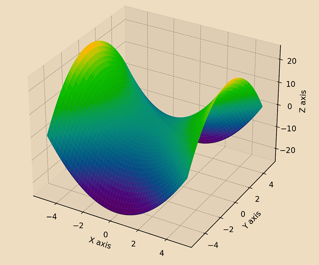
For this example, let’s use the example of a symplectic manifold and reduce this from 3D to 2D for simplicity using PCA.

The 3D shape:

Symplectic Manifold in 3D

The 2D shape:

PCA Reduced Symplectic Manifold to 2D

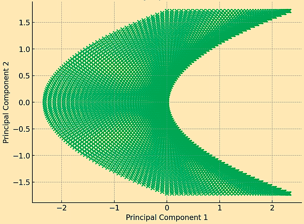
The scatterplot shows how the manifold, initially in three dimensions, is projected onto two principal components.

This process captures the essence of the manifold’s structure, focusing on the most significant variance directions.

By reducing the dimensionality, PCA provides a simplified view that can be more easily analyzed while retaining key features of the original manifold.

The code for doing this:

from sklearn.decomposition import PCA

# Define a grid
x = np.linspace(-5, 5, 100)
y = np.linspace(-5, 5, 100)
x, y = np.meshgrid(x, y)

# Define a symplectic form, e.g., a simple saddle as an example
z = x**2 - y**2

# Flatten the grid and z values for PCA
X_flat = x.flatten()
Y_flat = y.flatten()
Z_flat = z.flatten()

# Combine into a single data structure
data = np.vstack((X_flat, Y_flat, Z_flat)).T

# Standardize the data before applying PCA
scaler = StandardScaler()
data_standardized = scaler.fit_transform(data)

# Apply PCA
pca = PCA(n_components=2)
data_reduced = pca.fit_transform(data_standardized)

# Plot the reduced data
plt.figure(figsize=(8, 6))
plt.scatter(data_reduced[:, 0], data_reduced[:, 1], alpha=0.6, cmap='viridis')
plt.xlabel('Principal Component 1')
plt.ylabel('Principal Component 2')
plt.title('PCA Reduced Symplectic Manifold to 2D')
plt.grid(True)
plt.show()

Alternatives to PCA

Some alternatives to PCA analysis:

t-Distributed Stochastic Neighbor Embedding (t-SNE)

Effective for visualizing high-dimensional data in lower dimensions (especially 2D or 3D) by maintaining local data structures.

Independent Component Analysis (ICA)

Focuses on separating a multivariate signal into additive, independent components.

Useful for signal processing and time series analysis.

Factor Analysis (FA)

Identifies underlying variables (factors) that explain observed correlations among variables.

Uniform Manifold Approximation and Projection (UMAP)

A dimensionality reduction technique that maintains global data structure.

Useful for large datasets and better at preserving global structure than t-SNE.

Related

• UMAP and t-SNE in Manifold Learning (Trading Applications)
• UMAP and t-SNE in Topology (Trading Applications)

Conclusion

PCA simplifies the complexity inherent in financial markets, which allows for more focused and effective analysis.

While it comes with certain limitations, its benefits in risk management, market analysis, and model building make it an important and widely used technique in quantitative finance.

As with any analytical method, it should be used judiciously and in conjunction with other tools and domain knowledge to achieve the best results.