Manifold Learning in Finance, Markets & Trading

Manifold learning is a branch of machine learning that involves the analysis and understanding of high-dimensional data by finding low-dimensional representations without losing meaningful properties.

Key Takeaways – Manifold Learning in Finance, Markets & Trading

• Dimensionality Reduction
  • Manifold learning can simplify complex financial datasets.
  • Reveal underlying structures and relationships critical for informed trading decisions.
• Market Pattern Recognition
  • Helps in identifying non-linear patterns and trends in market data, essential for quant-driven trading strategies.
• Risk Assessment
  • Enhances risk management by providing deeper insights into asset behavior.
  • Helps traders to diversify and mitigate risks effectively.

This technique is valuable in finance for several reasons:

Dimensionality Reduction

Financial data often exist in high-dimensional spaces – i.e., there are many, many variables that impact economies and markets.

Manifold learning helps in reducing dimensionality.

This makes data analysis more manageable and less prone to overfitting.

Discovering Intrinsic Structures

It uncovers the intrinsic geometric structure of the data, which can be important for understanding complex/nuanced financial data.

For example, it can reveal hidden patterns in asset price movements or correlations.

Risk Management and Anomaly Detection

Manifold learning can help in detecting anomalies or changes in market behavior by identifying the fundamental structures in the data.

This is important for risk management.

Portfolio Optimization

It can enhance the process of portfolio construction by identifying underlying factors or market regimes that drive asset returns.

This can help in constructing portfolios that are better optimized for risk and return.

Algorithmic Trading

Manifold learning can help in developing more sophisticated trading algorithms by extracting and using complex features from market data, potentially leading to more profitable strategies.

Market Segmentation and Customer Insights

In retail finance, manifold learning can help in segmenting customers or products in a more nuanced manner.

This can lead to better-targeted products and marketing strategies.

Techniques in Manifold Learning

These techniques are particularly effective in visualizing high-dimensional data in lower dimensions (e.g., 2D or 3D) for exploratory data analysis.

Principal Component Analysis (PCA)

The most popular form of dimensionality reduction.

Simplifies data by reducing dimensions while retaining most variance.

Useful in identifying dominant market trends.

Isomap (Isometric Mapping)

Extends PCA.

Retains geometric relationships in data.

Ideal for uncovering intrinsic market structures obscured in high-dimensional space.

t-Distributed Stochastic Neighbor Embedding (t-SNE)

Visualizes high-dimensional data in lower dimensions.

Excellent for clustering and identifying patterns in complex financial datasets.

Uniform Manifold Approximation and Projection (UMAP)

Advanced technique for dimension reduction.

Efficient in revealing hidden structures and relationships in financial data.

Often outperforming t-SNE in speed and interpretability.

Locally Linear Embedding (LLE)

Preserves local relationships within data.

Good for modeling non-linear market dynamics where local similarities are important.

Autoencoders

Neural network-based approach for dimensionality reduction.

Effective in learning efficient representations of complex financial data.

Useful in anomaly detection and feature extraction.

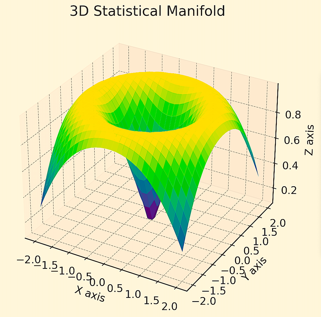
For instance, these might show multi-dimensional data in terms of a 3D manifold, like the below:

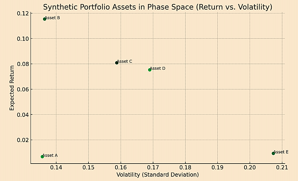
Or just in terms of a 2D structure plotting risk and return, which basically reduces dimensionality all the way down to the mean-variance framework:

Coding Example – Manifold Learning in Finance

Let’s try an optimization problem, as manifolds are commonly applied in finance.

To show some basic ideas, we can provide an example that touches on some of these concepts in a simplified way.

Example #1

We’ll visualize the efficient frontier in 3D (risk, return, and Sharpe Ratio), which can be seen as a type of geometric manifold. The efficient frontier represents a set of portfolios that offer the maximum expected return for a given level of risk.

In this 3D model, we can add the Sharpe Ratio (a measure of risk-adjusted return), to our previous plot of expected return versus volatility. This will allow us to visualize a 3D manifold that represents different portfolio characteristics.

We’ll use synthetic data for a set of assets, calculate the expected returns, volatilities, and correlations, and then use these to plot the efficient frontier:

import numpy as np 

import matplotlib.pyplot as plt 

from scipy.optimize import minimize

from mpl_toolkits.mplot3d import Axes3D

# Function to calculate the Sharpe Ratio
def sharpe_ratio(return_, volatility, risk_free_rate=0):
    return (return_ - risk_free_rate) / volatility

# Risk-free rate assumption (can be adjusted)
risk_free_rate = 0.01

# Calculate Sharpe Ratios for the target returns and volatilities
sharpe_ratios = [sharpe_ratio(tr, tv, risk_free_rate) for tr, tv in zip(target_returns, target_volatilities)]

# 3D plot of the efficient frontier
fig = plt.figure(figsize=(12, 8))
ax = fig.add_subplot(111, projection='3d')
ax.scatter(target_volatilities, target_returns, sharpe_ratios, c=sharpe_ratios, cmap='viridis')

ax.set_xlabel('Volatility')
ax.set_ylabel('Expected Return')
ax.set_zlabel('Sharpe Ratio')
ax.set_title('3D Efficient Frontier with Sharpe Ratios')
plt.show()

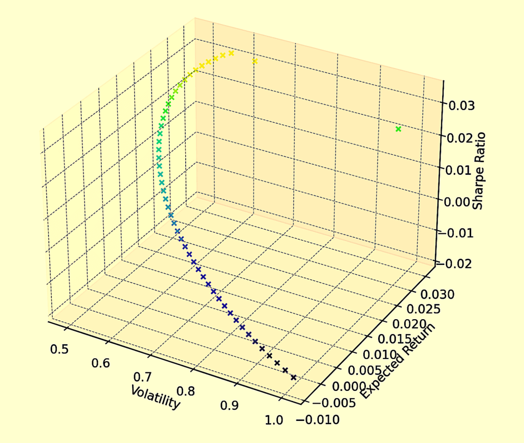
The color gradient, which represents different levels of the Sharpe Ratio, helps visualize the risk-adjusted return of each portfolio.

This 3D manifold-like representation offers a more nuanced view of the trade-offs between risk, return, and efficiency in portfolio optimization.

Example #2

The surface in this example represents combinations of volatility (x-axis), expected return (y-axis), and the Sharpe Ratio (z-axis).

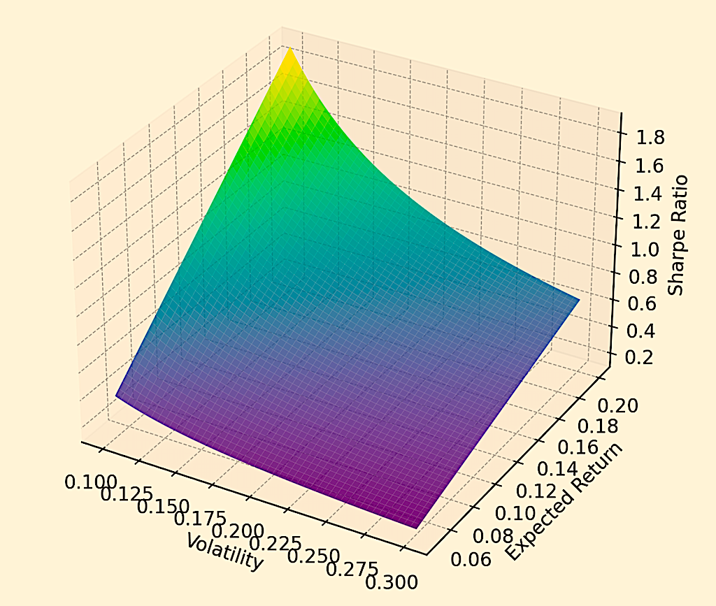
This geometric representation illustrates how these financial metrics interact and can provide a geometric understanding of the trade-offs involved in portfolio management and trading/investment strategies.

The curvature of the plane encapsulates the risk-adjusted return characteristics of different portfolio combinations.

We cover how to go about improving risk-reward in the article below.

Related

• Balanced Beta
• How to Build a Balanced Portfolio

The code to generate this graph:

import numpy as np
import matplotlib.pyplot as plt
from mpl_toolkits.mplot3d import Axes3D
from scipy.optimize import minimize

# Function to calculate the Sharpe Ratio
def sharpe_ratio(return_, volatility, risk_free_rate=0.01):
    return (return_ - risk_free_rate) / volatility

# Creating a meshgrid for the 3D surface
volatility_grid, return_grid = np.meshgrid(np.linspace(0.1, 0.3, 50), np.linspace(0.05, 0.2, 50))
sharpe_ratio_grid = sharpe_ratio(return_grid, volatility_grid)

# 3D plot
fig = plt.figure(figsize=(10, 7))
ax = fig.add_subplot(111, projection='3d')
ax.plot_surface(volatility_grid, return_grid, sharpe_ratio_grid, cmap='viridis', alpha=0.8)

ax.set_xlabel('Volatility')
ax.set_ylabel('Expected Return')
ax.set_zlabel('Sharpe Ratio')
ax.set_title('Risk-Return as a 3D Manifold')
plt.show()

Conclusion

In practice, the application of manifold learning in finance requires careful consideration of the nature of financial data, which often includes noise, non-stationarity, and non-linearity.

The choice of technique and its parameters should be aligned with the specific goals of the financial analysis or task at hand.