Uncorrelated ETFs


There are now thousands of different ETFs, with many of them providing different exposures to various parts of the market.
The main drawback, however, is that most of these ETFs are naturally equity funds.
And even if you’re in different sectors – e.g., tech ETF, consumer staples ETF, healthcare ETF – you know that stocks mostly go up and down together.
How do you get ETFs that are truly uncorrelated together, so you have returns streams that diversify and genuinely act independently of each other?
We’ll take a look.
Key Takeaways – Uncorrelated ETFs
- The overall purpose of uncorrelated ETFs is to introduce return streams into a portfolio.
- These should ideally be driven by different economic, structural, or physical forces so that portfolios perform better across a wider range of market environments rather than dependent on sustained growth or falling rates like most equity-centric (or bond-centric) portfolios.
- Stock ETFs give you broad exposure to economic growth and corporate earnings.
- But once you have a certain level of diversification among securities, buying more/having different ETFs doesn’t help as much because tend to move together during market ups or stress.
- Bond ETFs can offset equities during growth slowdowns or deflationary shocks.
- Their diversification benefit nonetheless weakens when inflation volatility dominates the macro drivers of returns.
- Gold ETFs offer long-term diversification against real rate declines and currency debasement, with return drivers largely independent of stocks and bonds.
- Commodity ETFs help hedge inflation (they’re sometimes the cause or a material contributor to inflation) and supply shocks.
- But such ETFs are often energy-heavy and less effective at diversifying pure growth risk.
- Some optimize roll yield to improve returns.
- CTA ETFs (Managed Futures) generate returns from trend-following across asset classes and can profit in rising or falling markets.
- This makes them among the most uncorrelated ETF strategies available.
- Merger Arbitrage ETFs get their returns from corporate deal completion rather than market direction.
- This generally results in low correlation to traditional asset classes over full cycles, though deals can fall apart during bad times, so it’s important to be mindful of that.
- Reinsurance and Insurance-Linked Securities ETFs are driven by catastrophe risk and insurance premiums.
- This introduces rare non-financial return drivers that are largely independent of economic conditions.
- Hedge Fund Strategy ETFs such as risk parity, market-neutral, or global macro try to diversify equity risk.
- The downside, though, is that they often retain partial correlation and have higher fees.
- Option-Based Income and Volatility ETFs earn returns from option premiums rather than price appreciation.
- They offer partial diversification that works best in flat or range-bound markets, given derivatives can customize returns in specific ways.
- This space is generally filled with covered call ETFs.
- Currency Strategy ETFs diversify portfolios through exposure to relative interest rates, capital flows, and policy differences rather than corporate profits or growth.
Stock ETFs
Stock ETFs are the foundation of most portfolios.
This generally includes a low-cost, highly liquid ETF that covers hundreds or thousands of securities in one fund.
Common examples include SPY, VOO, VT, and VTI. These are broad ETFs that cover US-focused large cap (SPY, VOO, VTI) or world large cap (VT).
There are also flavors related to size and style, such as large cap value (e.g., VTV), small cap value (e.g., VBR), US quality factor (e.g., VFQY), growth (e.g., VUG), and so on.
Bond ETFs
Bonds, particularly those with low/no credit risk, diversify stocks in certain environments, like when growth changes relative to expectations.
They don’t diversify when inflation is the dominant driver of returns. Both often fall together when inflation runs above expectations. 2022 was an example of why the negative stocks-bonds correlation is not reliable in all environments.
Also consider inflation-linked bonds, which can do a better job of providing real returns. They give you CPI (or some baseline inflation rate), plus a stated yield. At the same time, they still have interest rate risk.
There are many bond ETFs.
For low-credit risk ETFs of varying durations you can consider IEF, TLT, and BND.
For longer-duration corporate ETFs, consider LQD or VCLT.
Note that once you start taking on credit risk for extra yield – e.g., HYG, JNK – then you start correlating much more heavily to stocks, limiting diversification.
For inflation-linked securities, consider TIP, SCHP, or VTIP.
Gold ETFs
Gold has low long-run correlation with both stocks and bonds.
Its long-run valuation mirrors money growth (M0 or equivalent measures) well, though not necessarily over the short term.
At the same time, it’s generally not the best long-term investment, assuming the country’s currency is stable.
Its value is relative to the reference currency. In dollars, it’s returned a bit better than cash.
Always remember that gold is just gold. Its value reflects the world around it rather than its intrinsic value changing.
It helps to diversify stocks and bonds exposure over the long term due to its unique character. Protection against falling real rates and currency devaluation are its main qualities.
The GLD and IAU ETFs are most popular here.
Gold mining ETFs like GDX are equity-based and take on operational risk.
Commodity ETFs
Commodities don’t diversify stocks that well with respect to growth but can diversify with respect to inflation.
Commodity ETFs are nonetheless quite full of energy-linked commodities like oil and tend to not be very well balanced to things like agricultural commodities or softs.
GSG is a popular example, as is DBC.
Some commodity ETFs also try to optimize the roll process, as the strategy is typically effectuated through futures rather than physical ownership of the underlying commodities.
Instead of always holding the nearest futures contract – i.e., the “front month” – these strategies select contracts based on term structure and roll yield, favoring backwardated markets where the roll adds return and avoiding contangoed markets where rolling forward creates a persistent drag.
An example of a contango curve where the roll yield reduces profits:
And an example of a backwardated curve where the roll yield add profits:
An example of an optimization strategy here would involve calculating what maturity to own on the backwardated curve that gives the highest annualized return.
Not just the cheapest expiry, but the highest yield in annualized terms. So, not buying the flat part of the curve where the marginal roll is minimal.
A concrete example includes PDBC. This ETF dynamically chooses futures contracts across the curve to minimize negative roll and maximize carry while maintaining broad commodity exposure.
BCI is another. It uses an “optimum yield” methodology to hold the futures contract with the most favorable implied roll return rather than the front month.
Another example is COM. It applies a rules-based approach to contract selection and roll timing to reduce the structural losses from contango. Like most commodity ETFs, it mostly holds energy-heavy commodities like crude oil and natural gas.
These latter three ETFs still respond to supply-demand shocks and inflation. At the same time, their return profile is meaningfully different from traditional commodity ETFs such as GSG or DBC. A larger share of performance comes from futures curve economics rather than spot price changes alone.
CTA ETFs (Managed Futures)
CTA ETFs are among the closest things available in ETF form to a genuinely uncorrelated return stream.
These typically follow trend-following or systematic futures strategies across asset classes such as equities, bonds, commodities, and currencies.
Correlation tends to be low or even negative because shorting is a big part of the strategy.
Positions can be long or short (and you won’t know at any given time), and exposure shifts dynamically based on momentum and price trends rather than considerations like fundamentals or valuation.
This is important because CTA strategies don’t require markets to go up to make money.
They can perform well during sustained selloffs, inflationary shocks, commodity spikes, prolonged rate cycles, or any event where traditional portfolios will tend to struggle.
Historically, CTAs have shown their strongest diversification benefits during periods of equity stress, especially when markets experience extended directional moves rather than sharp mean reversion.
(Sharp mean reversion can actually catch CTA algorithms off guard, as they may not flips fast enough to go in the direction of the momentum.)
That makes them structurally different from stock or bond ETFs, which will heavily rely on economic growth or falling rates to keep churning out gains.
2022 was generally a good environment for them, when both stocks and bonds struggled and gold and commodities were a rather poor offset (especially given gold and commodities are lower-weighted in a portfolio).
At the same time, CTA returns can be cyclical and lumpy. They tend to struggle in choppy, range-bound markets where trends repeatedly reverse.
As a result, they often look disappointing during long bull markets but tend to do better when traditional portfolios are under pressure.
As an allocation, CTA ETFs work best as a structural diversifier, not as a tactical trade.
Their value lies in how they behave when other assets fail.
In ETF form, CTA and DBMF are the most popular.
Also note that these ETFs don’t have long histories.
So that we have data through the COVID-19 drop, we’ll exclude the CTA ETF and look at how DBMF correlated with other strategies.
Asset Correlations
| Name | Ticker | DBMF | SPY | IEF | TIP | GLD | GSG | Annualized Return | Daily Standard Deviation | Monthly Standard Deviation | Annualized Standard Deviation |
|---|---|---|---|---|---|---|---|---|---|---|---|
| iMGP DBi Managed Futures Strategy ETF | DBMF | 1.00 | -0.18 | -0.46 | -0.38 | -0.02 | 0.12 | 8.06% | 0.78% | 3.24% | 11.23% |
| SPDR S&P 500 ETF | SPY | -0.18 | 1.00 | 0.29 | 0.63 | 0.18 | 0.37 | 16.79% | 1.28% | 4.81% | 16.67% |
| iShares 7-10 Year Treasury Bond ETF | IEF | -0.46 | 0.29 | 1.00 | 0.78 | 0.40 | -0.32 | 0.56% | 0.47% | 2.11% | 7.32% |
| iShares TIPS Bond ETF | TIP | -0.38 | 0.63 | 0.78 | 1.00 | 0.44 | 0.05 | 2.83% | 0.42% | 1.68% | 5.80% |
| SPDR Gold Shares | GLD | -0.02 | 0.18 | 0.40 | 0.44 | 1.00 | -0.04 | 19.28% | 1.01% | 4.30% | 14.89% |
| iShares S&P GSCI Commodity-Indexed Trust | GSG | 0.12 | 0.37 | -0.32 | 0.05 | -0.04 | 1.00 | 6.98% | 1.48% | 6.42% | 22.25% |
| Asset correlations for time period 06/01/2019 – 11/30/2025 based on monthly returns | |||||||||||
We can see that it’s annualized return is pretty decent – 8.06% with low correlation across the board.
Of course, these are just average figures and the price history is short.
The fees associated with CTA ETFs are also high – commonly 0.75%-0.85% net expense ratios, or $75-$85 per year off every $10,000 invested.
Below you can see the rolling correlations to stocks (SPY) and bonds (IEF) over 36 months.
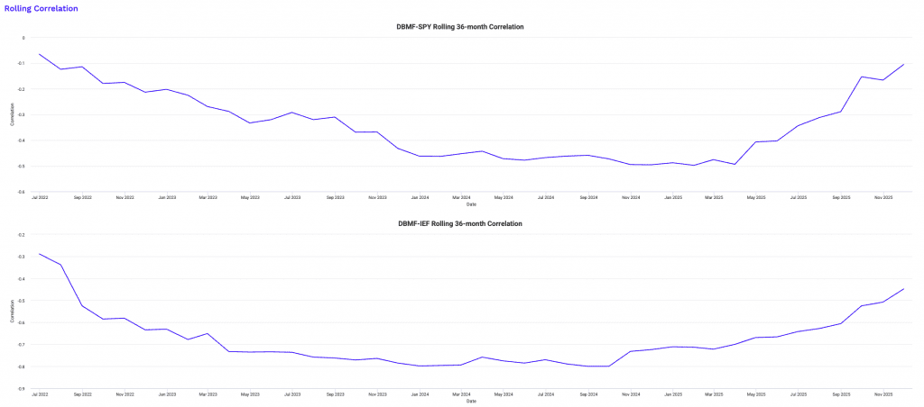
If we include the CTA ETF (which goes back to early 2022):
Asset Correlations
| Name | Ticker | CTA | DBMF | SPY | IEF | TIP | GLD | GSG | Annualized Return | Daily Standard Deviation | Monthly Standard Deviation | Annualized Standard Deviation |
|---|---|---|---|---|---|---|---|---|---|---|---|---|
| Simplify Managed Futures Strategy ETF | CTA | 1.00 | 0.57 | -0.36 | -0.59 | -0.41 | -0.51 | 0.19 | 9.74% | 0.96% | 4.48% | 15.51% |
| iMGP DBi Managed Futures Strategy ETF | DBMF | 0.57 | 1.00 | -0.42 | -0.62 | -0.57 | -0.28 | 0.19 | 5.24% | 0.73% | 3.65% | 12.63% |
| SPDR S&P 500 ETF | SPY | -0.36 | -0.42 | 1.00 | 0.64 | 0.75 | 0.15 | 0.25 | 13.49% | 1.13% | 4.66% | 16.15% |
| iShares 7-10 Year Treasury Bond ETF | IEF | -0.59 | -0.62 | 0.64 | 1.00 | 0.87 | 0.45 | -0.10 | 0.43% | 0.52% | 2.37% | 8.20% |
| iShares TIPS Bond ETF | TIP | -0.41 | -0.57 | 0.75 | 0.87 | 1.00 | 0.41 | 0.14 | 0.71% | 0.41% | 1.93% | 6.67% |
| SPDR Gold Shares | GLD | -0.51 | -0.28 | 0.15 | 0.45 | 0.41 | 1.00 | -0.03 | 23.18% | 1.01% | 4.18% | 14.49% |
| iShares S&P GSCI Commodity-Indexed Trust | GSG | 0.19 | 0.19 | 0.25 | -0.10 | 0.14 | -0.03 | 1.00 | 0.74% | 1.26% | 3.97% | 13.74% |
| Asset correlations for time period 04/01/2022 – 11/30/2025 based on monthly returns | ||||||||||||
We can see that both CTA ETFS (CTA and DBMF) correlate quite closely together.
What exactly is going on in these ETFs?
CTA ETFs probably drum up the most confusion of anything on this list.
What exactly are they doing in these things?
It’s natural, as after all, you want to know what your money is doing.
With a stock or bonds, you at least have a yield, income statement/balance sheet/CF statement, and so on to derive a yield.
Basically, CTA strategies run rules-based trend and momentum models on liquid futures markets. They express those signals mechanically.
Most fundamental is time-series momentum. The system looks at each market independently and asks a simple question: is price trending up or down over a defined lookback window?
Common horizons range from roughly three months to one year, often using multiple windows at the same time.
If crude oil has been rising consistently, the model goes long oil futures.
If 10-year Treasury futures have been falling, the model shorts them.
There’s no human forecast, narrative, or macro opinion involved.
Position sizing is volatility-targeted.
Each market is scaled so that it contributes a similar amount of risk to the portfolio.
A highly volatile contract like natural gas gets a much smaller position than fixed-duration positions that have structurally lower volatility – e.g., something like Eurodollar or Treasury futures.
This prevents any single market from dominating returns.
Risk is managed through combination of stop-outs and signal decay, not discretionary judgment.
If a trend weakens or reverses, exposure is reduced or flipped.
When markets move sideways and break trends repeatedly, positions churn and returns suffer.
When markets trend persistently, exposure grows and this is generally the best time for the strategy.
The DBMF strategy did okay through the 2020 COVID-19 drop, falling only modestly. It did really well during the 2022 sell-off.
The asset universe typically spans equity index futures, government bond futures across maturities, major commodities, and G10 currencies (USD, EUR, JPY, GBP, CAD, AUD, CHF, NZD, and possibly the Nordics NOK and SEK).
The strategy is always in a trade somewhere, but direction varies all the time.
Long equities in a bull market, short equities in a correction, bear market, or fall that meets the criteria. Long commodities during inflation spikes, short bonds during rate selloffs.
Importantly, CTA ETFs don’t try to time market tops or bottoms. It’s not an anticipatory strategy. It’s not “stocks are expensive, so I’m short” or “stocks are in a holding pattern after a long bull run, so time to flip short.”
It waits for confirmation.
They enter late and exit late by design.
But it’s still a bit different than day trading or standard swing trading.
The edge comes from capturing large, sustained moves that traditional portfolios struggle with, such as 2022’s simultaneous stock and bond drawdown.
CTAs are essentially geared toward option-like payoffs, where they take quick losses when trends are disconfirmed and make larger gains when trends bear themselves out.
In ETF form, vehicles like CTA and DBMF make use of these rules with daily liquidity, transparent holdings, and strict exposure limits, translating institutional managed futures programs into a regulated, systematic wrapper.
Merger Arbitrage ETFs
Merger arbitrage ETFs give exposure to corporate event risk rather than market direction.
These strategies typically invest in announced mergers and acquisitions. They buy the target company’s shares (which will increase if the deal closes) and hedge market exposure where possible.
Returns come from the spread between the current price and the deal’s expected closing value.
Because the payoff depends on deal completion rather than broad market performance, merger arb has historically shown low correlation to equities and bonds.
Market selloffs don’t automatically cause merger spreads to fail unless financing conditions or regulatory risk change materially.
That said, this of course isn’t a risk-free strategy and there is market expertise required.
Merger arb ETFs will generally bet on various deals without necessarily having explicit access to information that the market doesn’t.
Deal breaks, regulatory intervention, and funding stress can still lead to sharp losses.
The chance of this happening increases during bad periods, so you might expect some level of correlation to equities.
Correlations can rise temporarily during these periods.
Still, over full cycles, merger arbitrage behaves very differently from growth-driven assets. Returns are often modest but volatility tends to be pretty low.
This makes these ETFs more akin to an alternative income stream than a traditional risk asset.
At the same time, don’t expect it to materially beat cash without manager skill.
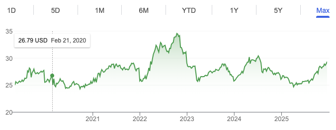
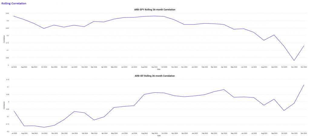
ARB is the most popular ETF here.
Asset Correlations
| Name | Ticker | ARB | SPY | IEF | Annualized Return | Daily Standard Deviation | Monthly Standard Deviation | Annualized Standard Deviation |
|---|---|---|---|---|---|---|---|---|
| AltShares Merger Arbitrage ETF | ARB | 1.00 | 0.31 | 0.07 | 4.60% | 0.28% | 0.94% | 3.25% |
| SPDR S&P 500 ETF | SPY | 0.31 | 1.00 | 0.51 | 17.53% | 1.09% | 4.50% | 15.58% |
| iShares 7-10 Year Treasury Bond ETF | IEF | 0.07 | 0.51 | 1.00 | -1.70% | 0.47% | 2.11% | 7.29% |
| Asset correlations for time period 06/01/2020 – 11/30/2025 based on monthly returns | ||||||||
Reinsurance and Insurance-Linked Securities ETFs
Reinsurance ETFs access one of the most structurally distinct sources of return available in public markets.
These funds invest in insurance-linked securities, often tied to catastrophe risk such as hurricanes, earthquakes, or other natural disasters. Returns are driven by insurance premiums and actuarial modeling rather than economic growth, earnings, or interest rates.
In most years, these strategies earn steady premium income. Losses occur when insured events exceed modeled expectations. Importantly, these events have no inherent connection to equity or bond markets.
That makes reinsurance exposure among the lowest-correlated assets available. A stock market crash doesn’t cause a hurricane, and a rally doesn’t prevent one.
The key risk is event clustering. A bad hurricane season or multiple disasters in a short period can produce drawdowns. Climate trends and changing weather patterns also introduce longer-term unknowns.
For diversification purposes, reinsurance ETFs are good because they introduce a non-financial risk driver into the portfolio. That’s rare and valuable.
The downside is that most investments in this space are private.
ILS is one example ETF in the space focusing on catastrophe (CAT) bonds, but it’s too new to really judge.
Asset Correlations
| Name | Ticker | ILS | SPY | IEF | Return | Daily Standard Deviation | Monthly Standard Deviation | Annualized Standard Deviation |
|---|---|---|---|---|---|---|---|---|
| Brookmont Catastrophic Bond ETF | ILS | 1.00 | 0.51 | -0.50 | 3.17% | 0.29% | 1.50% | 5.20% |
| SPDR S&P 500 ETF | SPY | 0.51 | 1.00 | -0.41 | 22.87% | 1.35% | 2.37% | 8.20% |
| iShares 7-10 Year Treasury Bond ETF | IEF | -0.50 | -0.41 | 1.00 | 4.89% | 0.35% | 1.02% | 3.53% |
| Asset correlations for time period 04/01/2025 – 11/30/2025 based on monthly returns | ||||||||
Hedge Fund Strategy ETFs
There are other hedge fund strategies outside of CTA/managed futures.
These generally have some correlation and many are more beta strategies by nature.
Examples – with example ETFs – include:
- Risk parity (e.g., ALLW)
- Market-neutral (e.g., BTAL)
- Global macro (e.g., HFGM, others)
- Levered beta (e.g., GDE, which is 90% stocks and 90% gold)
Many of these funds are new with not much data to them.
Also watch out for fees.
Let’s look at their correlations and returns with stocks and bonds:
ALLW
ALLW, a risk parity fund, has a fairly low correlation with equities but has shown higher correlation to bonds.
It was formerly institutional only, but is now in ETF form.
Asset Correlations
| Name | Ticker | ALLW | SPY | IEF | Return | Daily Standard Deviation | Monthly Standard Deviation | Annualized Standard Deviation |
|---|---|---|---|---|---|---|---|---|
| SPDR Bridgewater ALL Weather ETF | ALLW | 1.00 | 0.24 | 0.59 | 15.30% | 0.83% | 1.65% | 5.73% |
| SPDR S&P 500 ETF | SPY | 0.24 | 1.00 | -0.41 | 22.87% | 1.35% | 2.37% | 8.20% |
| iShares 7-10 Year Treasury Bond ETF | IEF | 0.59 | -0.41 | 1.00 | 4.89% | 0.35% | 1.02% | 3.53% |
| Asset correlations for time period 04/01/2025 – 11/30/2025 based on monthly returns | ||||||||
BTAL
BTAL has been around a while with negative correlation to equities, but has netted negative returns.
It’s effectively a hedge.
Asset Correlations
| Name | Ticker | BTAL | SPY | IEF | Annualized Return | Daily Standard Deviation | Monthly Standard Deviation | Annualized Standard Deviation |
|---|---|---|---|---|---|---|---|---|
| AGF U.S. Market Neutral Anti-Beta | BTAL | 1.00 | -0.62 | 0.17 | -2.94% | 1.04% | 4.22% | 14.62% |
| SPDR S&P 500 ETF | SPY | -0.62 | 1.00 | 0.06 | 15.57% | 1.07% | 4.06% | 14.06% |
| iShares 7-10 Year Treasury Bond ETF | IEF | 0.17 | 0.06 | 1.00 | 1.57% | 0.41% | 1.80% | 6.25% |
| Asset correlations for time period 10/01/2011 – 11/30/2025 based on monthly returns | ||||||||
HFGM
HFGM is a global macro ETF with a short history.
Asset Correlations
| Name | Ticker | HFGM | SPY | IEF | Return | Daily Standard Deviation | Monthly Standard Deviation | Annualized Standard Deviation |
|---|---|---|---|---|---|---|---|---|
| Unlimited HFGM Global Macro ETF | HFGM | 1.00 | 0.18 | 0.45 | 25.76% | 1.25% | 3.23% | 11.20% |
| SPDR S&P 500 ETF | SPY | 0.18 | 1.00 | -0.38 | 23.94% | 0.76% | 2.05% | 7.10% |
| iShares 7-10 Year Treasury Bond ETF | IEF | 0.45 | -0.38 | 1.00 | 3.79% | 0.32% | 1.08% | 3.75% |
| Asset correlations for time period 05/01/2025 – 11/30/2025 based on monthly returns | ||||||||
GDE
As mentioned, GDE is 180% gross exposure, split between stocks and gold.
Asset Correlations
| Name | Ticker | GDE | SPY | IEF | Annualized Return | Daily Standard Deviation | Monthly Standard Deviation | Annualized Standard Deviation |
|---|---|---|---|---|---|---|---|---|
| WisdomTree Efcnt Gld Pls Eq Stgy ETF | GDE | 1.00 | 0.78 | 0.71 | 29.43% | 1.58% | 5.97% | 20.69% |
| SPDR S&P 500 ETF | SPY | 0.78 | 1.00 | 0.64 | 13.49% | 1.13% | 4.66% | 16.15% |
| iShares 7-10 Year Treasury Bond ETF | IEF | 0.71 | 0.64 | 1.00 | 0.43% | 0.52% | 2.37% | 8.20% |
| Asset correlations for time period 04/01/2022 – 11/30/2025 based on monthly returns | ||||||||
Note that GDE’s returns are not sustainable long term at this level. It simply generally coincides with a good to great period for each asset class (stocks and gold).
Other Diversifying ETF Categories Worth Considering
Beyond the major alternatives above, there are several other ETF types that can provide partial or situational diversification.
Market-Neutral and Long-Short Equity ETFs attempt to isolate stock selection skill while minimizing market beta. Correlation is lower than long-only equities, though not zero, and performance depends heavily on manager execution.
An example would be the above-mentioned BTAL.
Commodity Carry and Roll-Optimized ETFs differ from simple commodity spot exposure by harvesting futures curve dynamics. These strategies are more sensitive to supply-demand imbalances than growth cycles.
PBDC, BCI, and COM would be examples.
Volatility and Option-Based Income ETFs generate returns through option premiums rather than price appreciation. They’re not fully uncorrelated, their return drivers still differ meaningfully from equity beta, especially in flat or sideways markets.
JEPI would be an example, which sells covered calls against equities.
You can see JEPI’s high correlation with equities and how it tends to underperform in stronger periods for equities due to the capped upside.
Asset Correlations
| Name | Ticker | JEPI | SPY | IEF | Annualized Return | Daily Standard Deviation | Monthly Standard Deviation | Annualized Standard Deviation |
|---|---|---|---|---|---|---|---|---|
| JPMorgan Equity Premium Income ETF | JEPI | 1.00 | 0.89 | 0.48 | 11.38% | 0.69% | 2.98% | 10.34% |
| SPDR S&P 500 ETF | SPY | 0.89 | 1.00 | 0.51 | 17.53% | 1.09% | 4.50% | 15.58% |
| iShares 7-10 Year Treasury Bond ETF | IEF | 0.48 | 0.51 | 1.00 | -1.70% | 0.47% | 2.11% | 7.29% |
| Asset correlations for time period 06/01/2020 – 11/30/2025 based on monthly returns | ||||||||
Currency Strategy ETFs, particularly those focused on carry, value, or momentum across FX markets, can add diversification because currencies respond to relative policy, trade balances, and capital flows rather than corporate earnings.
Each of these comes with tradeoffs. None are perfect substitutes for one another, and none are guaranteed diversifiers in all environments.
Putting It Together
True diversification comes from independent economic drivers, not just different tickers.
As examples…
CTA ETFs diversify through price trends across asset classes. Merger arb ETFs diversify through deal mechanics. Reinsurance ETFs diversify through physical risk events.
When combined thoughtfully with stocks, bonds, and real assets, these strategies help build portfolios that perform better across a wider range of outcomes rather than optimized for a single environment like most portfolios (i.e., toward strong growth).
Overall, that is the real purpose of uncorrelated ETFs.
Related: Uncorrelated Strategies
Appendix: Why Uncorrelated ETFs Improve Risk-Adjusted Returns
When a portfolio has assets that cover different economic drivers, it can perform better in a wider range of environments.
Consider the following three portfolios:
Portfolio 1 – Stocks Only
| Asset Class | Allocation |
|---|---|
| US Stock Market | 100.00% |
Portfolio 2 – Stocks + Bonds
| Asset Class | Allocation |
|---|---|
| US Stock Market | 40.00% |
| 10-year Treasury | 60.00% |
Portfolio 3 – Stocks + Bonds + Gold
| Asset Class | Allocation |
|---|---|
| US Stock Market | 40.00% |
| 10-year Treasury | 40.00% |
| Gold | 20.00% |
Portfolio 1 is most concentrated.
Portfolio 2 adds bonds.
Portfolio 3 adds the unique return-additive and risk-reducing exposure of gold.
Here’s the performance snapshot:
Performance Summary
| Metric | Portfolio 1 | Portfolio 2 | Portfolio 3 |
|---|---|---|---|
| Start Balance | $10,000 | $10,000 | $10,000 |
| End Balance | $2,614,786 | $854,125 | $1,379,230 |
| Annualized Return (CAGR) | 10.88% | 8.60% | 9.57% |
| Standard Deviation | 15.63% | 8.16% | 8.52% |
| Best Year | 37.82% | 31.94% | 35.74% |
| Worst Year | -37.04% | -16.96% | -14.07% |
| Maximum Drawdown | -50.89% | -19.39% | -18.16% |
| Sharpe Ratio | 0.46 | 0.51 | 0.59 |
| Sortino Ratio | 0.66 | 0.78 | 0.92 |
Portfolio 2 adds bonds.
Portfolio 3 adds the unique return-additive and risk-reducing exposure of gold.
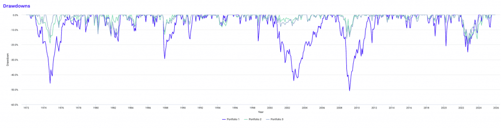
Notice how the maximum drawdown and risk-adjusted return metrics (Sharpe, Sortino) go up the better diversified the portfolio is.
Here, you can see the steep yearly drawdowns that occur with concentrated portfolios and the shallow ones of diversified portfolios.
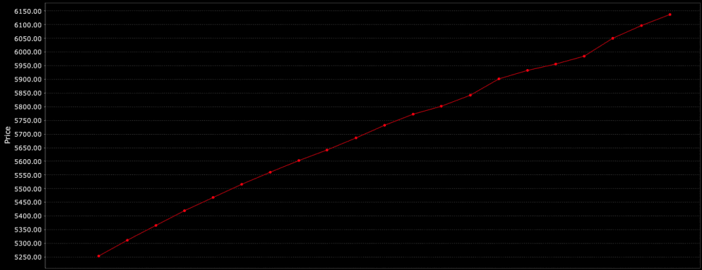
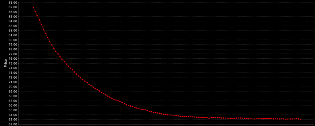
This can provide another visual:
Some fuller, more detailed statistics:
Risk and Return Metrics
| Metric | Portfolio 1 | Portfolio 2 | Portfolio 3 |
|---|---|---|---|
| Arithmetic Mean (monthly) | 0.97% | 0.72% | 0.79% |
| Arithmetic Mean (annualized) | 12.24% | 8.96% | 9.96% |
| Geometric Mean (monthly) | 0.86% | 0.69% | 0.76% |
| Geometric Mean (annualized) | 10.88% | 8.60% | 9.57% |
| Standard Deviation (monthly) | 4.51% | 2.36% | 2.46% |
| Standard Deviation (annualized) | 15.63% | 8.16% | 8.52% |
| Downside Deviation (monthly) | 2.92% | 1.33% | 1.37% |
| Maximum Drawdown | -50.89% | -19.39% | -18.16% |
| Benchmark Correlation | 1.00 | 0.80 | 0.76 |
| Beta(*) | 1.00 | 0.42 | 0.41 |
| Alpha (annualized) | 0.00% | 3.75% | 4.72% |
| R2 | 100.00% | 64.34% | 57.94% |
| Sharpe Ratio | 0.46 | 0.51 | 0.59 |
| Sortino Ratio | 0.66 | 0.78 | 0.92 |
| Treynor Ratio (%) | 7.14 | 9.90 | 12.22 |
| Calmar Ratio | 2.16 | 1.38 | 2.74 |
| Modigliani–Modigliani Measure | 11.60% | 12.42% | 13.77% |
| Active Return | 0.00% | -2.28% | -1.31% |
| Tracking Error | 0.00% | 10.31% | 10.68% |
| Information Ratio | N/A | -0.22 | -0.12 |
| Skewness | -0.52 | -0.04 | -0.12 |
| Excess Kurtosis | 1.90 | 1.15 | 1.50 |
| Historical Value-at-Risk (5%) | 7.05% | 3.25% | 3.18% |
| Analytical Value-at-Risk (5%) | 6.45% | 3.16% | 3.25% |
| Conditional Value-at-Risk (5%) | 9.93% | 4.56% | 4.47% |
| Upside Capture Ratio (%) | 100.00 | 48.20 | 50.14 |
| Downside Capture Ratio (%) | 100.00 | 35.22 | 32.80 |
| Safe Withdrawal Rate | 4.29% | 3.90% | 5.40% |
| Perpetual Withdrawal Rate | 6.39% | 4.39% | 5.25% |
| Positive Periods | 406 out of 647 (62.75%) | 425 out of 647 (65.69%) | 420 out of 647 (64.91%) |
| Gain/Loss Ratio | 1.03 | 1.17 | 1.24 |
| * US Stock Market is used as the benchmark for calculations. Value-at-risk metrics are monthly values. | |||
How these portfolios did during historical stress periods:
Historical Market Stress Periods
| Stress Period | Start | End | Portfolio 1 | Portfolio 2 | Portfolio 3 |
|---|---|---|---|---|---|
| Oil Crisis | Oct 1973 | Mar 1974 | -12.61% | -5.98% | -2.97% |
| Black Monday Period | Sep 1987 | Nov 1987 | -29.34% | -13.23% | -11.33% |
| Asian Crisis | Jul 1997 | Jan 1998 | -3.72% | -2.67% | -2.45% |
| Russian Debt Default | Jul 1998 | Oct 1998 | -17.57% | -5.13% | -7.38% |
| Dotcom Crash | Mar 2000 | Oct 2002 | -44.11% | -5.55% | -7.94% |
| Subprime Crisis | Nov 2007 | Mar 2009 | -50.89% | -13.39% | -15.92% |
| COVID-19 Start | Jan 2020 | Mar 2020 | -20.89% | -4.02% | -5.57% |
For portfolio 1 (stocks only), you can see the depth of the drawdowns:
Drawdowns for Portfolio 1
| Rank | Start | End | Length | Recovery By | Recovery Time | Underwater Period | Drawdown |
|---|---|---|---|---|---|---|---|
| 1 | Nov 2007 | Feb 2009 | 1 year 4 months | Mar 2012 | 3 years 1 month | 4 years 5 months | -50.89% |
| 2 | Jan 1973 | Sep 1974 | 1 year 9 months | Dec 1976 | 2 years 3 months | 4 years | -45.86% |
| 3 | Sep 2000 | Sep 2002 | 2 years 1 month | Apr 2006 | 3 years 7 months | 5 years 8 months | -44.11% |
| 4 | Sep 1987 | Nov 1987 | 3 months | May 1989 | 1 year 6 months | 1 year 9 months | -29.34% |
| 5 | Jan 2022 | Sep 2022 | 9 months | Dec 2023 | 1 year 3 months | 2 years | -24.94% |
| 6 | Jan 2020 | Mar 2020 | 3 months | Jul 2020 | 4 months | 7 months | -20.89% |
| 7 | Dec 1980 | Jul 1982 | 1 year 8 months | Oct 1982 | 3 months | 1 year 11 months | -17.85% |
| 8 | Jul 1998 | Aug 1998 | 2 months | Nov 1998 | 3 months | 5 months | -17.57% |
| 9 | Jun 1990 | Oct 1990 | 5 months | Feb 1991 | 4 months | 9 months | -16.20% |
| 10 | Oct 2018 | Dec 2018 | 3 months | Apr 2019 | 4 months | 7 months | -14.28% |
| Worst 10 drawdowns included above | |||||||
Shallower for portfolio 2, given fixed-duration bonds are added and shifted away from stocks, but also due to the diversifying effects:
Drawdowns for Portfolio 2
| Rank | Start | End | Length | Recovery By | Recovery Time | Underwater Period | Drawdown |
|---|---|---|---|---|---|---|---|
| 1 | Jan 2022 | Sep 2022 | 9 months | Jul 2024 | 1 year 10 months | 2 years 7 months | -19.39% |
| 2 | Jan 1973 | Sep 1974 | 1 year 9 months | Jun 1975 | 9 months | 2 years 6 months | -19.05% |
| 3 | Dec 2007 | Feb 2009 | 1 year 3 months | Sep 2009 | 7 months | 1 year 10 months | -13.39% |
| 4 | Sep 1987 | Nov 1987 | 3 months | Oct 1988 | 11 months | 1 year 2 months | -13.23% |
| 5 | Sep 1979 | Mar 1980 | 7 months | May 1980 | 2 months | 9 months | -9.74% |
| 6 | Jun 1981 | Sep 1981 | 4 months | Nov 1981 | 2 months | 6 months | -9.34% |
| 7 | Feb 1994 | Jun 1994 | 5 months | Mar 1995 | 9 months | 1 year 2 months | -8.24% |
| 8 | Jul 1983 | May 1984 | 11 months | Aug 1984 | 3 months | 1 year 2 months | -7.92% |
| 9 | Jul 1975 | Sep 1975 | 3 months | Dec 1975 | 3 months | 6 months | -6.51% |
| 10 | Aug 1990 | Sep 1990 | 2 months | Dec 1990 | 3 months | 5 months | -6.42% |
| Worst 10 drawdowns included above | |||||||
And when adding gold:
Drawdowns for Portfolio 3
| Rank | Start | End | Length | Recovery By | Recovery Time | Underwater Period | Drawdown |
|---|---|---|---|---|---|---|---|
| 1 | Jan 2022 | Sep 2022 | 9 months | Mar 2024 | 1 year 6 months | 2 years 3 months | -18.16% |
| 2 | Mar 2008 | Oct 2008 | 8 months | Sep 2009 | 11 months | 1 year 7 months | -15.92% |
| 3 | Apr 1974 | Sep 1974 | 6 months | Feb 1975 | 5 months | 11 months | -15.18% |
| 4 | Dec 1980 | Sep 1981 | 10 months | Sep 1982 | 1 year | 1 year 10 months | -14.36% |
| 5 | Feb 1980 | Mar 1980 | 2 months | Jun 1980 | 3 months | 5 months | -12.90% |
| 6 | Sep 1987 | Nov 1987 | 3 months | Apr 1989 | 1 year 5 months | 1 year 8 months | -11.33% |
| 7 | Jul 1975 | Sep 1975 | 3 months | Jan 1976 | 4 months | 7 months | -8.69% |
| 8 | Jul 1983 | May 1984 | 11 months | Oct 1984 | 5 months | 1 year 4 months | -7.97% |
| 9 | Sep 2000 | Mar 2001 | 7 months | May 2003 | 2 years 2 months | 2 years 9 months | -7.94% |
| 10 | Jul 1998 | Aug 1998 | 2 months | Oct 1998 | 2 months | 4 months | -7.38% |
| Worst 10 drawdowns included above | |||||||
Some statistics on individual assets:
Portfolio Assets
| Name | CAGR | Stdev | Best Year | Worst Year | Max Drawdown | Sharpe Ratio | Sortino Ratio |
|---|---|---|---|---|---|---|---|
| US Stock Market | 10.88% | 15.63% | 37.82% | -37.04% | -50.89% | 0.46 | 0.66 |
| 10-year Treasury | 6.30% | 8.02% | 39.57% | -15.19% | -23.18% | 0.25 | 0.38 |
| Gold | 8.67% | 19.59% | 126.55% | -32.60% | -61.78% | 0.29 | 0.49 |
Monthly correlations of each asset to each other and each of the three portfolio constructions:
Monthly Correlations
| Name | US Stock Market | 10-year Treasury | Gold | Portfolio 1 | Portfolio 2 | Portfolio 3 |
|---|---|---|---|---|---|---|
| US Stock Market | 1.00 | 0.07 | 0.02 | 1.00 | 0.80 | 0.76 |
| 10-year Treasury | 0.07 | 1.00 | 0.08 | 0.07 | 0.65 | 0.47 |
| Gold | 0.02 | 0.08 | 1.00 | 0.02 | 0.07 | 0.54 |
Portfolio Risk Decomposition
| Name | Portfolio 1 | Portfolio 2 | Portfolio 3 |
|---|---|---|---|
| US Stock Market | 100.00% | 61.69% | 56.92% |
| 10-year Treasury | 38.31% | 17.96% | |
| Gold | 25.12% | ||
| Risk attribution decomposes portfolio risk into its constituent parts and identifies the contribution to overall volatility by each of the assets. | |||
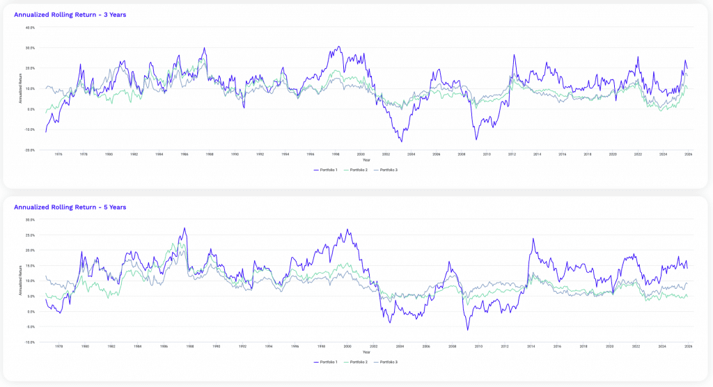
Rolling returns really show the benefits.
Note the continuous red with the all-stocks portfolio (at a point lasting more than a decade, and we’ve seen multiple decades in cases like Japan).
But this thins out with better diversified portfolios:
Rolling Returns
| Roll Period | Portfolio 1 | Portfolio 2 | Portfolio 3 | ||||||
|---|---|---|---|---|---|---|---|---|---|
| Average | High | Low | Average | High | Low | Average | High | Low | |
| 1 year | 12.08% | 66.73% | -43.18% | 8.93% | 48.02% | -17.15% | 9.69% | 47.16% | -15.10% |
| 3 years | 11.31% | 30.70% | -16.27% | 8.85% | 24.63% | -2.12% | 9.24% | 22.45% | -0.58% |
| 5 years | 11.41% | 27.25% | -6.23% | 9.04% | 22.27% | 1.95% | 9.28% | 19.64% | 2.93% |
| 7 years | 11.37% | 21.23% | -3.02% | 9.16% | 18.84% | 3.72% | 9.31% | 15.53% | 5.15% |
| 10 years | 11.30% | 18.89% | -2.57% | 9.33% | 15.92% | 3.85% | 9.23% | 14.85% | 4.78% |
| 15 years | 11.07% | 18.21% | 4.25% | 9.41% | 14.66% | 5.58% | 9.20% | 13.27% | 6.06% |