Optimal Leverage Ratio for a Diversified Beta Portfolio


In institutional settings, and for advanced individual traders, beta portfolios are often given a slight boost with leverage.
This is often done with futures or other derivatives (e.g., options) that embed institutional borrowing rates (rather than paying retail markups).
But what is the optimal leverage ratio?
Too little gives you modest returns. Too much exposes you to excess volatility and drawdowns.
We’ll take a look using simulations and data from past history, simulating a balanced portfolio of stocks (S&P 500), bonds (10-year Treasury), and gold.
Key Takeaways – Optimal Leverage Ratio for a Diversified Beta Portfolio
- 1x (No leverage):
- Stable, diversified growth.
- Shallow drawdowns and strong behavioral durability.
- But it feels “underpowered” and capital efficiency is low.
- Long-term returns remain capped relative to what the portfolio structure can support.
- 1.5x leverage:
- Improves return efficiency meaningfully while also keeping volatility, drawdowns, and recovery times within a range most disciplined traders/investors can tolerate.
- Inflation-driven correlation spikes still create 27-28% drawdowns.
- 2x leverage:
- Pushes historical returns into 14-15% annualized territory with equity-like volatility but with improved risk-adjusted metrics and strong compounding.
- But drawdowns move into the mid-30% range and performance drag from the funding costs impact the portfolio.
- 2.5x leverage:
- Produces very high long-run returns and preserves diversification benefits statistically.
- Yet drawdowns routinely exceed 40%.
- At this level, considerations like funding stability, rebalancing discipline, and psychological endurance are critical constraints.
- Tail risk protection becomes more important.
- 3x leverage:
- Maximizes compounding power with ~20% CAGRs and strong upside capture.
- Statistically, it works. But it introduces 50% drawdowns and multi-year underwater periods.
- Survival, liquidity/funding access and stability, and sequencing risk dominate all other considerations.
- The optimal leverage is the highest level you can hold through the portfolio’s worst historical drawdowns and longest underwater periods without forced de-risking.
- ~1.5x–2.0x is a practical sweet spot for most sophisticated traders/investors.
- 2.5x+ is reserved for truly stable financing and institutional-grade risk controls.
- It also depends a lot on the exact construction of the portfolio and of course what risk controls are in place. The more diversified and reliable the returns streams, the more the portfolio structure can support.
- The decision ultimately depends on the exact nature of the portfolio, your drawdown tolerance, funding/borrowing cost and stability, ability to rebalance in stress, time horizon, and whether you can withstand correlation breakdowns without capitulating.
- Leverage is generally done with futures, options, or any access to risk-free interest rate borrowing, not with sources with high spreads/markups.
1x (No) Leverage
Let’s try a standard portfolio with no leverage. Just the basic positions.
Here are our allocations.
We’ll use these throughout the bulk of the article.
Portfolio 1
| Asset Class | Allocation |
|---|---|
| US Stock Market | 40.00% |
| 10-year Treasury | 50.00% |
| Gold | 10.00% |
Portfolio 2
| Asset Class | Allocation |
|---|---|
| US Stock Market | 40.00% |
| 10-year Treasury | 45.00% |
| Gold | 15.00% |
“Portfolio 2” throughout will be a slightly heavier allocation to gold.
Performance Summary
Performance summary statistics in this article run from 1972 to the present:
| Metric | Portfolio 1 | Portfolio 2 |
|---|---|---|
| Start Balance | $10,000 | $10,000 |
| End Balance | $1,106,309 | $1,240,912 |
| Annualized Return (CAGR) | 9.12% | 9.35% |
| Standard Deviation | 8.05% | 8.22% |
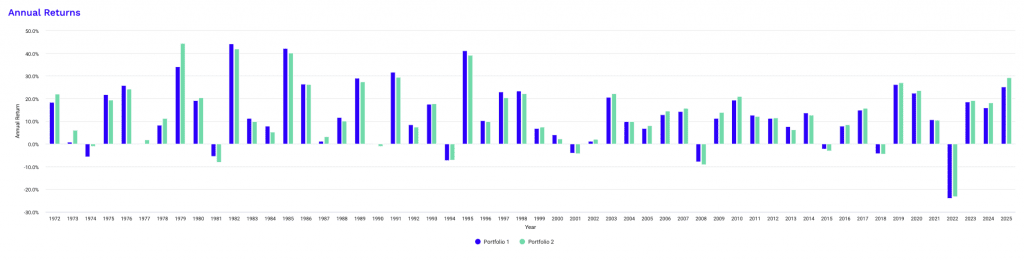
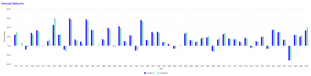
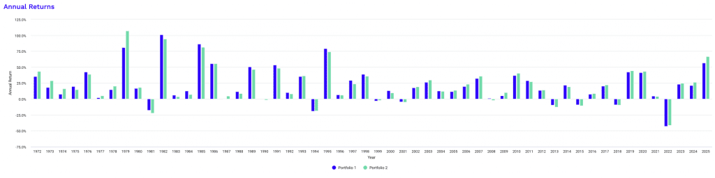
| Best Year | 29.48% | 29.50% |
| Worst Year | -15.51% | -14.79% |
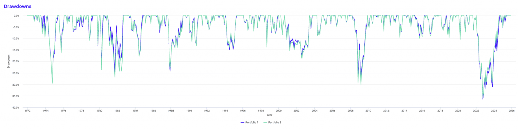
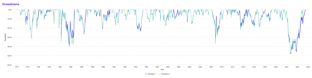
| Maximum Drawdown | -18.77% | -18.46% |
| Sharpe Ratio | 0.57 | 0.59 |
| Sortino Ratio | 0.88 | 0.91 |
The 1x leverage performance summary gives us a clear baseline for how an unlevered diversified beta portfolio behaves over a full market cycle.
Using data from 1972 to the present and a $10,000 starting balance, both portfolios give steady long-term growth with controlled risk.
Portfolio 1 grows to approximately $1.11 million, while Portfolio 2 reaches about $1.24 million. The difference is driven primarily by Portfolio 2’s slightly higher exposure to gold, which improves performance during inflationary and crisis periods without materially increasing volatility. This shows up in the higher CAGR of 9.35% versus 9.12% for Portfolio 1.
Both portfolios being north of 9% is actually quite good.
Volatility remains modest for both portfolios. Standard deviation sits just above 8% in each case, which is materially lower than an equity-only portfolio over the same period – by about 50%.
Getting more than a unit of return per each unit of volatility is always good.
Best and worst calendar-year returns are also very similar.
In all this, you can kind of see that once the portfolio has a certain structure, changing things up by 1-5% doesn’t meaningfully increase upside or downside extremes.
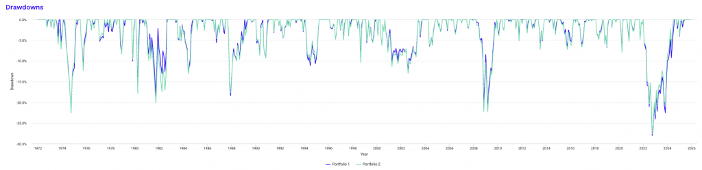
Drawdowns are well-contained. Maximum drawdowns remain below 19% for both portfolios, a level that many investors can tolerate without forced deleveraging (not part of this because we aren’t using leverage here) or behavioral errors.
Risk-adjusted metrics reinforce this idea. Portfolio 2 posts slightly higher Sharpe and Sortino ratios, reflecting marginally better return efficiency per unit of total and downside risk.
Overall, these results show that a diversified, unlevered beta portfolio produces stable returns with limited drawdowns.
But it also highlights why institutions often consider adding leverage to improve capital efficiency.
Risk and Return Metrics
| Metric | Portfolio 1 | Portfolio 2 |
|---|---|---|
| Arithmetic Mean (monthly) | 0.76% | 0.78% |
| Arithmetic Mean (annualized) | 9.47% | 9.72% |
| Geometric Mean (monthly) | 0.73% | 0.75% |
| Geometric Mean (annualized) | 9.12% | 9.35% |
| Standard Deviation (monthly) | 2.33% | 2.37% |
| Standard Deviation (annualized) | 8.05% | 8.22% |
| Downside Deviation (monthly) | 1.31% | 1.33% |
| Maximum Drawdown | -18.77% | -18.46% |
| Benchmark Correlation | 0.81 | 0.79 |
| Beta(*) | 0.42 | 0.42 |
| Alpha (annualized) | 4.25% | 4.49% |
| R2 | 65.43% | 62.50% |
| Sharpe Ratio | 0.57 | 0.59 |
| Sortino Ratio | 0.88 | 0.91 |
| Treynor Ratio (%) | 11.08 | 11.66 |
| Calmar Ratio | 1.99 | 2.35 |
| Modigliani–Modigliani Measure | 13.44% | 13.69% |
| Active Return | -1.75% | -1.52% |
| Tracking Error | 10.27% | 10.43% |
| Information Ratio | -0.17 | -0.15 |
| Skewness | -0.12 | -0.14 |
| Excess Kurtosis | 1.21 | 1.30 |
| Historical Value-at-Risk (5%) | 3.10% | 3.18% |
| Analytical Value-at-Risk (5%) | 3.07% | 3.13% |
| Conditional Value-at-Risk (5%) | 4.37% | 4.36% |
| Upside Capture Ratio (%) | 49.25 | 49.71 |
| Downside Capture Ratio (%) | 33.91 | 33.33 |
| Safe Withdrawal Rate | 4.65% | 5.03% |
| Perpetual Withdrawal Rate | 4.86% | 5.06% |
| Positive Periods | 424 out of 647 (65.53%) | 418 out of 647 (64.61%) |
| Gain/Loss Ratio | 1.22 | 1.27 |
| * US Stock Market is used as the benchmark for calculations. Value-at-risk metrics are monthly values. | ||
This expanded metric set gives us a more granular view of how each portfolio behaves across different dimensions of risk, return, and benchmark interaction.
The distinction between arithmetic and geometric returns has to do with the volatility drag inherent in multi-asset portfolios, with the gap remaining small due to relatively low variance.
Monthly dispersion stays contained, which reinforces the stability of return paths over time.
Downside-focused measures clarify portfolio behavior in adverse conditions.
Downside deviation and value-at-risk estimates remain tightly clustered between the two portfolios, so they have similar short-term loss characteristics.
Benchmark-related statistics show important structural differences. Both portfolios have low beta relative to the US equity market, which is good, as it’s important that they function as true diversified beta portfolios rather than equity proxies.
Alpha remains positive in both cases; this isn’t true alpha in terms of deviating from a benchmark. But it does suggest returns in excess of what equity exposure alone would imply, even after accounting for volatility.
Lower R² values reinforce that a substantial portion of returns comes from non-equity sources.
Capture ratios show asymmetric participation, which is key in diversified portfolios.
Upside capture remains below 50%, while downside capture is materially lower. This shows effective loss mitigation during equity market declines, given much of the portfolio is in bonds and gold, which respond to their own economic influences.
Distributional metrics show mild negative skewness and moderate excess kurtosis, consistent with occasional stress events but not extreme tail behavior.
Withdrawal metrics and gain-loss ratios show durable cash flow potential, with Portfolio 2 showing slightly stronger sustainability for long-horizon spending despite similar win rates.
Historical Market Stress Periods
| Stress Period | Start | End | Portfolio 1 | Portfolio 2 |
|---|---|---|---|---|
| Oil Crisis | Oct 1973 | Mar 1974 | -3.49% | -3.22% |
| Black Monday Period | Sep 1987 | Nov 1987 | -12.26% | -11.79% |
| Asian Crisis | Jul 1997 | Jan 1998 | -2.56% | -2.51% |
| Russian Debt Default | Jul 1998 | Oct 1998 | -6.25% | -6.82% |
| Dotcom Crash | Mar 2000 | Oct 2002 | -6.50% | -7.12% |
| Subprime Crisis | Nov 2007 | Mar 2009 | -13.65% | -14.60% |
| COVID-19 Start | Jan 2020 | Mar 2020 | -4.80% | -5.18% |
The historical stress period figures we have above show how each portfolio responds during well-known episodes of market dislocation rather than in normal/averaged-out conditions.
Across most crises, drawdowns remain shallow relative to equity-only benchmarks.
This shows the stabilizing effect of bonds and gold during systemic shocks.
Bonds are good for deflationary/disinflationary shocks while gold is good during geopolitical strife when trust between countries is lower and currency devaluation is ongoing.
During the 1973-1974 oil crisis and the Asian financial crisis, losses stay limited to low single digits. This shows the protective value of duration and non-cyclical assets.
The 1987 Black Monday episode stands out as the sharpest short-term shock, yet drawdowns remain contained near the low teens, far below the equity market collapse of that period.
Differences between the two portfolios are modest and context-dependent.
Portfolio 2 performs slightly better during inflation-sensitive and abrupt shock events, while Portfolio 1 gives you marginally better performance in select deflationary or bond-friendly environments.
Longer drawdowns such as the dotcom crash and the subprime crisis show the benefit of diversification over extended equity bear markets.
Both portfolios avoided the deep, prolonged capital impairment seen in stocks alone.
Overall, the results show that diversified beta portfolios do better in crisis drawdowns versus being in just one asset class (especially equities, given their strong growth sensitivity).
They create a more stable foundation for considering leverage without immediately increasing tail risk.
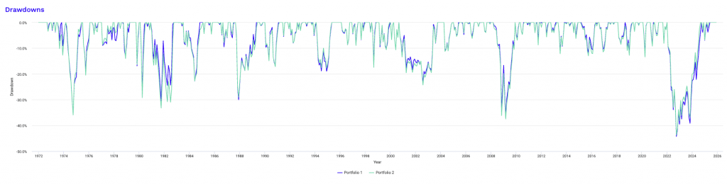
Drawdowns for Portfolio 1
| Rank | Start | End | Length | Recovery By | Recovery Time | Underwater Period | Drawdown |
|---|---|---|---|---|---|---|---|
| 1 | Jan 2022 | Sep 2022 | 9 months | Jun 2024 | 1 year 9 months | 2 years 6 months | -18.77% |
| 2 | Mar 1974 | Sep 1974 | 7 months | Feb 1975 | 5 months | 1 year | -15.02% |
| 3 | Mar 2008 | Feb 2009 | 1 year | Sep 2009 | 7 months | 1 year 7 months | -13.65% |
| 4 | Sep 1987 | Nov 1987 | 3 months | Jan 1989 | 1 year 2 months | 1 year 5 months | -12.26% |
| 5 | Dec 1980 | Sep 1981 | 10 months | Aug 1982 | 11 months | 1 year 9 months | -11.78% |
| 6 | Feb 1980 | Mar 1980 | 2 months | May 1980 | 2 months | 4 months | -10.91% |
| 7 | Jul 1983 | May 1984 | 11 months | Sep 1984 | 4 months | 1 year 3 months | -7.93% |
| 8 | Jul 1975 | Sep 1975 | 3 months | Jan 1976 | 4 months | 7 months | -7.59% |
| 9 | Feb 1994 | Jun 1994 | 5 months | Mar 1995 | 9 months | 1 year 2 months | -7.14% |
| 10 | Oct 1979 | Oct 1979 | 1 month | Dec 1979 | 2 months | 3 months | -6.60% |
| Worst 10 drawdowns included above | |||||||
The 2022 drawdown is notable because it occurred during a regime in which traditional diversification did poorly.
Inflation-driven tightening caused stocks and long-duration bonds to decline at the same time, eliminating the negative correlation that typically stabilizes stock-bond portfolios. This had been reliable since the early 1990s.
Unlike crisis-driven selloffs where bonds provide immediate ballast, rising yields directly impaired Treasury returns while equities repriced lower in response to tighter financial conditions.
Gold provided only partial offset during the early phase of the shock.
As a result, Portfolio 1 experienced its deepest drawdown at -18.77%, with losses extending over nine months and a prolonged recovery period.
Diversifying does tend to help shorten underwater periods since the drawdowns stay relatively shallow and they tend to recover in a more stable way.
This episode highlights that diversified beta portfolios remain vulnerable when macro forces compress cross-asset correlations, an important consideration when evaluating leverage during inflationary tightening cycles.
Drawdowns for Portfolio 2
| Rank | Start | End | Length | Recovery By | Recovery Time | Underwater Period | Drawdown |
|---|---|---|---|---|---|---|---|
| 1 | Jan 2022 | Sep 2022 | 9 months | Mar 2024 | 1 year 6 months | 2 years 3 months | -18.46% |
| 2 | Mar 1974 | Sep 1974 | 7 months | Feb 1975 | 5 months | 1 year | -15.08% |
| 3 | Mar 2008 | Oct 2008 | 8 months | Sep 2009 | 11 months | 1 year 7 months | -14.60% |
| 4 | Dec 1980 | Sep 1981 | 10 months | Aug 1982 | 11 months | 1 year 9 months | -13.08% |
| 5 | Feb 1980 | Mar 1980 | 2 months | Jun 1980 | 3 months | 5 months | -11.92% |
| 6 | Sep 1987 | Nov 1987 | 3 months | Jan 1989 | 1 year 2 months | 1 year 5 months | -11.79% |
| 7 | Jul 1975 | Sep 1975 | 3 months | Jan 1976 | 4 months | 7 months | -8.14% |
| 8 | Jul 1983 | May 1984 | 11 months | Oct 1984 | 5 months | 1 year 4 months | -7.95% |
| 9 | Sep 2000 | Mar 2001 | 7 months | May 2003 | 2 years 2 months | 2 years 9 months | -7.12% |
| 10 | Jul 1998 | Aug 1998 | 2 months | Oct 1998 | 2 months | 4 months | -6.82% |
| Worst 10 drawdowns included above | |||||||
Similar results seen here.
Portfolio Assets
Some statistics on the building blocks we’re using:
| Name | CAGR | Stdev | Best Year | Worst Year | Max Drawdown | Sharpe Ratio | Sortino Ratio |
|---|---|---|---|---|---|---|---|
| US Stock Market | 10.88% | 15.63% | 37.82% | -37.04% | -50.89% | 0.46 | 0.66 |
| 10-year Treasury | 6.30% | 8.02% | 39.57% | -15.19% | -23.18% | 0.25 | 0.38 |
| Gold | 8.67% | 19.59% | 126.55% | -32.60% | -61.78% | 0.29 | 0.49 |
The component-level statistics show why diversification is essential before considering leverage.
US equities deliver the highest long-term growth but also have severe drawdowns and volatility.
This makes them capital inefficient on a standalone basis.
There’s also a question of whether 10.9% CAGR is a realistic long-term return. 6-8% is a more normal outcome.
Treasuries provide stability and lower drawdowns, though with reduced return potential.
Gold shows the most extreme dispersion, with episodic outsized gains and deep elongated drawdowns. It’s more of a convex hedge rather than a steady return generator.
Individually, none of these assets offer very attractive risk-adjusted performance.
Their value emerges through combination, where imperfect correlations transform volatile components into a smoother, more durable return profile suitable for controlled leverage.
Monthly Correlations
| Name | US Stock Market | 10-year Treasury | Gold | Portfolio 1 | Portfolio 2 |
|---|---|---|---|---|---|
| US Stock Market | 1.00 | 0.07 | 0.02 | 0.81 | 0.79 |
| 10-year Treasury | 0.07 | 1.00 | 0.08 | 0.58 | 0.52 |
| Gold | 0.02 | 0.08 | 1.00 | 0.32 | 0.44 |
The correlation matrix shows the average correlations – a measure of diversification.
Stocks, Treasuries, and gold show low pairwise correlations, allowing risk to be spread.
Portfolio correlations with equities remain well below one.
The slightly higher gold weight in Portfolio 2 lowers equity linkage further while increasing diversification benefits.
These low correlations are the foundation that makes modest leverage viable, as risk scales more slowly than returns when assets don’t move together.
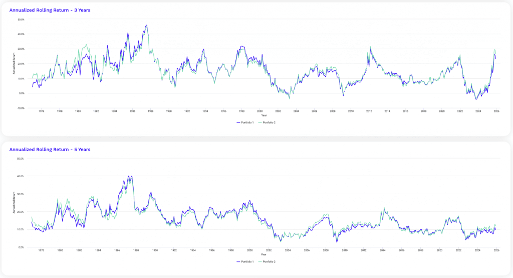
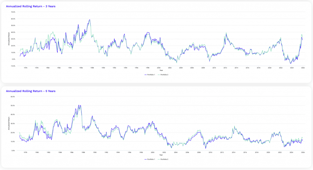
3-Year and 5-Year Rolling Returns
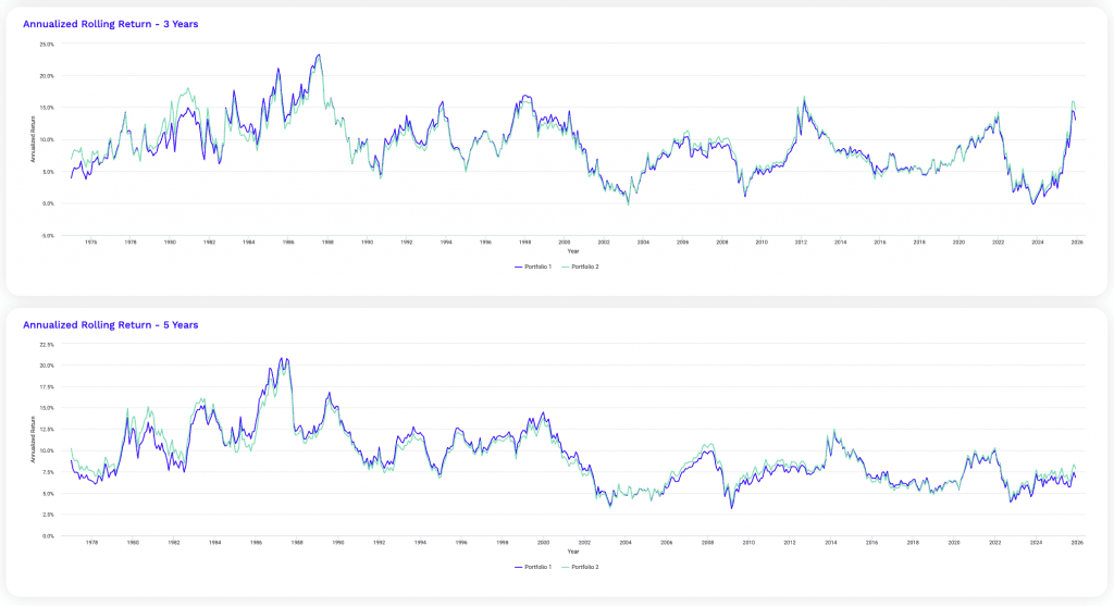
The rolling return profiles show how portfolio performance runs across multiple years rather than just one single year – which can be noisy.
Three-year rolling returns naturally show wider dispersion, with pronounced swings during inflationary cycles, equity booms, and policy-driven drawdowns.
This shorter horizon shows sequencing risk and highlights periods where returns temporarily compress or surge.
Five-year rolling returns are materially smoother, as more time allows for markets’ returns to converge to the risk premiums merited.
Extended drawdowns tend to mean-revert as bonds and gold reassert their hedging roles.
The close tracking between portfolios reinforces that small allocation shifts primarily affect return consistency at the margins.
1.5x Leverage
Same portfolios:
Portfolio 1
| Asset Class | Allocation |
|---|---|
| US Stock Market | 40.00% |
| 10-year Treasury | 50.00% |
| Gold | 10.00% |
Portfolio 2
| Asset Class | Allocation |
|---|---|
| US Stock Market | 40.00% |
| 10-year Treasury | 45.00% |
| Gold | 15.00% |
Performance Summary
| Metric | Portfolio 1 | Portfolio 2 |
|---|---|---|
| Start Balance | $10,000 | $10,000 |
| End Balance | $4,535,300 | $5,356,062 |
| Annualized Return (CAGR) | 12.01% | 12.36% |
| Standard Deviation | 12.08% | 12.33% |
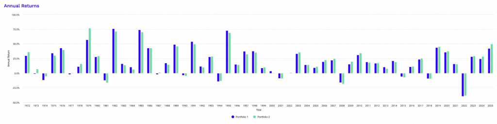
| Best Year | 44.07% | 44.27% |
| Worst Year | -24.04% | -23.05% |
| Maximum Drawdown | -28.04% | -27.61% |
| Sharpe Ratio | 0.64 | 0.65 |
| Sortino Ratio | 0.99 | 1.02 |
At 1.5x leverage, the portfolios move into a materially different return regime while remaining within a range that many institutional allocators would still consider controllable.
The increase in capital efficiency is immediately visible. A $10,000 starting balance compounds to approximately $4.5 million for Portfolio 1 and $5.36 million for Portfolio 2. This is a substantial step up from the unlevered case.
Annualized returns rise into the low-12% range, while volatility increases proportionally into the low-12% band. (Leverage cost assumptions in each case is 3% per turn in each portfolio in this analysis.)
Importantly, risk-adjusted performance improves rather than deteriorates.
Both Sharpe and Sortino ratios are higher than at 1x. So, leverage is still operating in a zone where diversification benefits dominate volatility drag.
Drawdowns deepen but remain bounded. Maximum drawdowns of roughly 28% are meaningfully larger than the unlevered case, yet far from what you see with equity-only portfolios.
Worst-year losses remain tolerable and occur during the same macro regimes identified earlier, particularly periods of correlation breakdown.
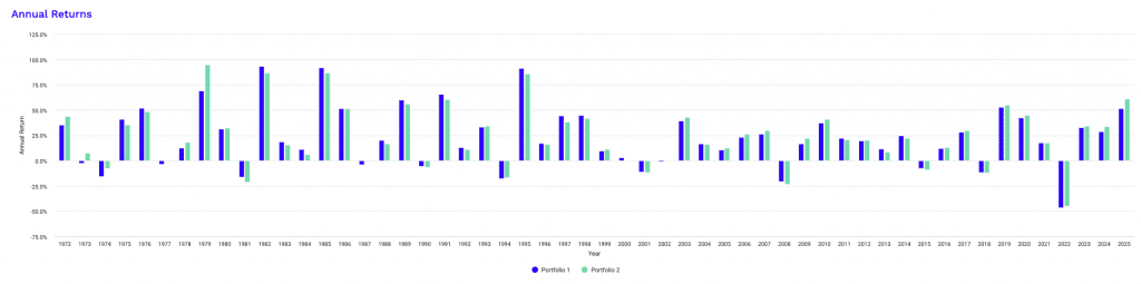
You’ll notice in the graph below that the worst year in the sample was 2022 because of correlations running together. It was materially worse than 2008, the 2000-02 period, tighter monetary policy periods (1981, 1994), and any of th evolatile 1970s years.
Portfolio 2 continues to show slightly superior efficiency, providing higher returns with marginally lower drawdowns.
Overall, 1.5x leverage sits near a practical inflection point where returns scale faster than risk and drawdowns remain manageable.
This sets a strong benchmark for evaluating whether additional leverage is justified.
Risk and Return Metrics
| Metric | Portfolio 1 | Portfolio 2 |
|---|---|---|
| Arithmetic Mean (monthly) | 1.01% | 1.04% |
| Arithmetic Mean (annualized) | 12.82% | 13.20% |
| Geometric Mean (monthly) | 0.95% | 0.98% |
| Geometric Mean (annualized) | 12.01% | 12.36% |
| Standard Deviation (monthly) | 3.49% | 3.56% |
| Standard Deviation (annualized) | 12.08% | 12.33% |
| Downside Deviation (monthly) | 2.02% | 2.05% |
| Maximum Drawdown | -28.04% | -27.61% |
| Benchmark Correlation | 0.81 | 0.79 |
| Beta(*) | 0.63 | 0.62 |
| Alpha (annualized) | 4.87% | 5.23% |
| R2 | 65.43% | 62.50% |
| Sharpe Ratio | 0.64 | 0.65 |
| Sortino Ratio | 0.99 | 1.02 |
| Treynor Ratio (%) | 12.25 | 12.83 |
| Calmar Ratio | 1.80 | 2.14 |
| Modigliani–Modigliani Measure | 14.41% | 14.64% |
| Active Return | 1.14% | 1.48% |
| Tracking Error | 9.21% | 9.57% |
| Information Ratio | 0.12 | 0.16 |
| Skewness | -0.12 | -0.14 |
| Excess Kurtosis | 1.21 | 1.30 |
| Historical Value-at-Risk (5%) | 4.78% | 4.90% |
| Analytical Value-at-Risk (5%) | 4.73% | 4.82% |
| Conditional Value-at-Risk (5%) | 6.68% | 6.67% |
| Upside Capture Ratio (%) | 72.15 | 72.87 |
| Downside Capture Ratio (%) | 54.25 | 53.44 |
| Safe Withdrawal Rate | 6.85% | 7.72% |
| Perpetual Withdrawal Rate | 7.36% | 7.64% |
| Positive Periods | 416 out of 647 (64.30%) | 412 out of 647 (63.68%) |
| Gain/Loss Ratio | 1.17 | 1.21 |
| * US Stock Market is used as the benchmark for calculations. Value-at-risk metrics are monthly values. | ||
The expanded statistics at 1.5x leverage clarify how risk scales across multiple dimensions beyond headline volatility.
Monthly arithmetic returns move above 1%, while the gap between arithmetic and geometric means widens modestly. This reflects increased volatility drag that remains manageable.
Importantly, the dispersion between monthly and annualized figures stays contained. This suggests that leverage doesn’t meaningfully destabilize compounding efficiency at this level.
Benchmark sensitivity increases but remains restrained. Beta rises into the low-0.6 range, confirming that leverage amplifies equity exposure without turning the portfolios into equity substitutes.
R² values remain well below 70%, so a large share of return variance still originates from non-equity sources.
Positive alpha expands, but this just has to do with diversified factor exposure.
Downside metrics provide additional context. Monthly downside deviation increases, yet capture ratios remain asymmetric.
Upside capture rises into the low-70% range, while downside capture stays materially lower. So the portfolio’s defensive asymmetry is still high.
Calmar ratios – most commonly used with commodity funds – remain elevated, which show that return gains outpace drawdown expansion even as absolute losses deepen.
Tail risk measures move higher in absolute terms but do so proportionally. Historical and analytical value-at-risk metrics remain tightly aligned, which suggest stable return distributions rather than model distortion from leverage.
Conditional value-at-risk rises, but not disproportionately, indicating that tail outcomes are amplified rather than structurally altered.
Tracking error declines slightly relative to return gains, lifting information ratios into positive territory. This implies improved efficiency versus the benchmark despite higher leverage.
Withdrawal metrics improve materially, pointing to stronger sustainability for income-oriented mandates.
Overall, the data indicate that 1.5x leverage enhances return quality across multiple risk lenses without introducing instability typical of higher leverage regimes.
Historical Market Stress Periods
| Stress Period | Start | End | Portfolio 1 | Portfolio 2 |
|---|---|---|---|---|
| Oil Crisis | Oct 1973 | Mar 1974 | -5.35% | -4.96% |
| Black Monday Period | Sep 1987 | Nov 1987 | -18.41% | -17.75% |
| Asian Crisis | Jul 1997 | Jan 1998 | -3.97% | -3.89% |
| Russian Debt Default | Jul 1998 | Oct 1998 | -9.57% | -10.41% |
| Dotcom Crash | Mar 2000 | Oct 2002 | -12.32% | -13.02% |
| Subprime Crisis | Nov 2007 | Mar 2009 | -21.55% | -22.37% |
| COVID-19 Start | Jan 2020 | Mar 2020 | -7.39% | -7.96% |
Stress-period drawdowns at 1.5x leverage show predictable amplification.
Losses deepen proportionally across all events, but the relative ordering of stress severity remains consistent with the unlevered case, of course, because we didn’t change the allocation.
Also factor in the drag from the interest cost of leverage (1.5% in this case, with half a turn of leverage at a 3% cost assumption).
Inflation-driven shocks and sudden liquidity events produce the sharpest declines, while region-specific crises remain well contained.
Importantly, drawdowns stay materially below equity-only losses during the same periods, confirming that diversification continues to function even under leverage.
Differences between the two portfolios remain modest and event-dependent, with gold-weighted Portfolio 2 slightly better in inflationary shocks and marginally weaker during deflationary recessions.
These results show that moderate leverage increases magnitude, not fragility.
Drawdowns for Portfolio 1
| Rank | Start | End | Length | Recovery By | Recovery Time | Underwater Period | Drawdown |
|---|---|---|---|---|---|---|---|
| 1 | Jan 2022 | Sep 2022 | 9 months | Jul 2024 | 1 year 10 months | 2 years 7 months | -28.04% |
| 2 | Mar 1974 | Sep 1974 | 7 months | Apr 1975 | 7 months | 1 year 2 months | -22.49% |
| 3 | Mar 2008 | Feb 2009 | 1 year | Nov 2009 | 9 months | 1 year 9 months | -21.55% |
| 4 | Dec 1980 | Sep 1981 | 10 months | Aug 1982 | 11 months | 1 year 9 months | -18.41% |
| 5 | Sep 1987 | Nov 1987 | 3 months | Jan 1989 | 1 year 2 months | 1 year 5 months | -18.41% |
| 6 | Feb 1980 | Mar 1980 | 2 months | May 1980 | 2 months | 4 months | -16.37% |
| 7 | Jul 1983 | May 1984 | 11 months | Oct 1984 | 5 months | 1 year 4 months | -13.05% |
| 8 | Sep 2000 | Jul 2002 | 1 year 11 months | May 2003 | 10 months | 2 years 9 months | -12.32% |
| 9 | Jul 1975 | Sep 1975 | 3 months | Jan 1976 | 4 months | 7 months | -11.59% |
| 10 | Feb 1994 | Jun 1994 | 5 months | Mar 1995 | 9 months | 1 year 2 months | -11.16% |
| Worst 10 drawdowns included above | |||||||
The worst drawdowns for Portfolio 1 at 1.5x leverage shows how leverage reshapes the depth and duration of capital impairment without fundamentally changing recovery dynamics.
The 2022 inflation-driven tightening cycle remains the most severe episode, producing a near 28% drawdown and an extended underwater period exceeding two and a half years.
This shows that correlation convergence is the biggest threat to such portfolios. Namely, assets we assume are mostly uncorrelated correlating during certain stress events.
Earlier macro shocks, including the 1970s inflation regime and the global financial crisis, also deepen materially but retain recovery timelines broadly consistent with the unlevered portfolio.
Notably, recovery times do not scale linearly with drawdown depth.
Several double-digit drawdowns recover within a year, while others with similar magnitudes remain underwater far longer due to macro persistence rather than leverage itself.
Equity crashes driven by valuation resets and policy shifts tend to prolong recoveries more than short, liquidity-driven shocks.
These results emphasize that leverage increases patience requirements rather than fragility.
Investors will have to tolerate deeper interim losses and longer psychological stress, even though long-term capital recovery remains intact under diversified exposure.
Drawdowns for Portfolio 2
| Rank | Start | End | Length | Recovery By | Recovery Time | Underwater Period | Drawdown |
|---|---|---|---|---|---|---|---|
| 1 | Jan 2022 | Sep 2022 | 9 months | Jun 2024 | 1 year 9 months | 2 years 6 months | -27.61% |
| 2 | Mar 1974 | Sep 1974 | 7 months | Feb 1975 | 5 months | 1 year | -22.58% |
| 3 | Mar 2008 | Feb 2009 | 1 year | Nov 2009 | 9 months | 1 year 9 months | -22.37% |
| 4 | Dec 1980 | Sep 1981 | 10 months | Sep 1982 | 1 year | 1 year 10 months | -20.22% |
| 5 | Feb 1980 | Mar 1980 | 2 months | Jun 1980 | 3 months | 5 months | -17.87% |
| 6 | Sep 1987 | Nov 1987 | 3 months | Apr 1989 | 1 year 5 months | 1 year 8 months | -17.75% |
| 7 | Jul 1983 | May 1984 | 11 months | Oct 1984 | 5 months | 1 year 4 months | -13.06% |
| 8 | Sep 2000 | Jul 2002 | 1 year 11 months | May 2003 | 10 months | 2 years 9 months | -13.02% |
| 9 | Jul 1975 | Sep 1975 | 3 months | Jan 1976 | 4 months | 7 months | -12.39% |
| 10 | Jul 1998 | Aug 1998 | 2 months | Oct 1998 | 2 months | 4 months | -10.41% |
| Worst 10 drawdowns included above | |||||||
2x Leverage
Again, same portfolios:
Portfolio 1
| Asset Class | Allocation |
|---|---|
| US Stock Market | 40.00% |
| 10-year Treasury | 50.00% |
| Gold | 10.00% |
Portfolio 2
| Asset Class | Allocation |
|---|---|
| US Stock Market | 40.00% |
| 10-year Treasury | 45.00% |
| Gold | 15.00% |
Performance Summary
| Metric | Portfolio 1 | Portfolio 2 |
|---|---|---|
| Start Balance | $10,000 | $10,000 |
| End Balance | $17,007,254 | $21,063,630 |
| Annualized Return (CAGR) | 14.79% | 15.25% |
| Standard Deviation | 16.11% | 16.44% |
| Best Year | 59.57% | 60.06% |
| Worst Year | -32.06% | -30.85% |
| Maximum Drawdown | -36.52% | -36.00% |
| Sharpe Ratio | 0.67 | 0.68 |
| Sortino Ratio | 1.05 | 1.08 |
At this higher 2x leverage level, or $1 borrowed for every $1 in our own money, the portfolios enter a setup where return maximization and risk tolerance become tightly coupled.
Compounding accelerates dramatically, with ending balances reaching roughly $17.0 million for Portfolio 1 and over $21.0 million for Portfolio 2 from the same $10,000 starting point.
Annualized returns move into the mid-teens, placing these portfolios in a performance tier typically associated with concentrated equity exposure, yet achieved through diversified beta rather than single-asset class risk.
Because of the leverage cost, our return comes in at slightly less than one percentage point for each perfect point of volatility, as expressed as a standard deviation.
Volatility rises meaningfully into the mid-16% range, which is about standard for US equities. But risk-adjusted metrics continue to improve incrementally. Sharpe and Sortino ratios are higher than at lower leverage levels because of the relative performance relative to cash.
This shows that incremental leverage still converts diversification into usable return. Portfolio 2, with the higher gold, again demonstrates slightly superior efficiency, pairing higher returns with marginally lower downside severity.
Drawdowns deepen to the mid-30% range, which materially changes the experience for the trader/investor.
Worst calendar-year losses exceed 30%, and maximum drawdowns approach levels that can force behavioral capitulation or mechanical deleveraging if capital buffers are insufficient.
So here there’s a practical boundary where leverage shifts from being primarily an efficiency tool to a structural risk decision.
Best-year returns near 60% highlight the convex upside embedded in leveraged diversification during favorable regimes, particularly falling-rate and reflationary environments.
At the same time, recovery discipline becomes essential, as large gains are paired with long and psychologically taxing drawdown cycles.
Overall, this leverage level remains mathematically attractive. But it will nonetheless require institutional-grade risk management, stable funding, and the ability to remain invested through severe but temporary capital impairment.
Risk and Return Metrics
| Metric | Portfolio 1 | Portfolio 2 |
|---|---|---|
| Arithmetic Mean (monthly) | 1.26% | 1.30% |
| Arithmetic Mean (annualized) | 16.27% | 16.79% |
| Geometric Mean (monthly) | 1.16% | 1.19% |
| Geometric Mean (annualized) | 14.79% | 15.25% |
| Standard Deviation (monthly) | 4.65% | 4.75% |
| Standard Deviation (annualized) | 16.11% | 16.44% |
| Downside Deviation (monthly) | 2.72% | 2.77% |
| Maximum Drawdown | -36.52% | -36.00% |
| Benchmark Correlation | 0.81 | 0.79 |
| Beta(*) | 0.83 | 0.83 |
| Alpha (annualized) | 5.49% | 5.97% |
| R2 | 65.43% | 62.50% |
| Sharpe Ratio | 0.67 | 0.68 |
| Sortino Ratio | 1.05 | 1.08 |
| Treynor Ratio (%) | 12.84 | 13.42 |
| Calmar Ratio | 1.71 | 2.05 |
| Modigliani–Modigliani Measure | 14.89% | 15.11% |
| Active Return | 3.92% | 4.37% |
| Tracking Error | 9.82% | 10.41% |
| Information Ratio | 0.40 | 0.42 |
| Skewness | -0.12 | -0.14 |
| Excess Kurtosis | 1.21 | 1.30 |
| Historical Value-at-Risk (5%) | 6.45% | 6.61% |
| Analytical Value-at-Risk (5%) | 6.38% | 6.51% |
| Conditional Value-at-Risk (5%) | 8.99% | 8.98% |
| Upside Capture Ratio (%) | 96.04 | 97.02 |
| Downside Capture Ratio (%) | 74.36 | 73.35 |
| Safe Withdrawal Rate | 8.93% | 10.46% |
| Perpetual Withdrawal Rate | 9.64% | 10.00% |
| Positive Periods | 411 out of 647 (63.52%) | 410 out of 647 (63.37%) |
| Gain/Loss Ratio | 1.16 | 1.17 |
| * US Stock Market is used as the benchmark for calculations. Value-at-risk metrics are monthly values. | ||
At 2x leverage, the portfolios reach a zone where leverage meaningfully alters portfolio behavior rather than simply scaling it.
Return statistics remain compelling.
Arithmetic and geometric returns stay well aligned, indicating that compounding efficiency has not yet collapsed under volatility drag.
The persistence of positive alpha and stable R² suggests that diversified factor exposure continues to drive returns rather than pure equity beta, even as beta approaches the mid-0.8 range (the stocks part is being levered to being almost 1x capital).
Several advantages stand out at this level. Upside capture approaches parity with the equity market, meaning the portfolio increasingly participates in strong bull regimes while still maintaining diversification.
Information ratios improve further, showing that excess returns over the benchmark are becoming more consistent rather than episodic.
Withdrawal metrics rise sharply, showing that for investors with stable funding and long horizons, cash-flow sustainability meaningfully improves.
Importantly, skewness and kurtosis remain relatively stable, implying that leverage hasn’t introduced structurally new tail behavior.
But here, costs become more visible. Downside capture climbs materially, reducing the asymmetry that defined lower leverage regimes.
Tail risk measures rise into a range where monthly losses during stress events can challenge margin tolerance and liquidity planning.
Calmar ratios flatten or decline, which denote that drawdown depth is beginning to compete with return gains.
While drawdowns remain recoverable historically, recovery paths become increasingly sensitive to macro factors rather than cyclical mean reversion.
Whether leverage should increase further depends on the trader or investor’s constraints.
For institutions with long-dated liabilities, low funding costs, and disciplined rebalancing, marginal increases beyond 2x may still be defensible, though expected benefits narrow. For most allocators, this level represents a practical ceiling.
Many institutional risk parity/levered beta portfolios are around 2x leverage.
Below 2x, leverage improves efficiency; above it, leverage increasingly converts diversification into path dependency.
The optimal decision here is less about maximizing returns and more about survival through prolonged correlation breakdowns without forced deleveraging.
Historical Market Stress Periods
| Stress Period | Start | End | Portfolio 1 | Portfolio 2 |
|---|---|---|---|---|
| Oil Crisis | Oct 1973 | Mar 1974 | -7.22% | -6.70% |
| Black Monday Period | Sep 1987 | Nov 1987 | -24.33% | -23.50% |
| Asian Crisis | Jul 1997 | Jan 1998 | -5.37% | -5.27% |
| Russian Debt Default | Jul 1998 | Oct 1998 | -12.85% | -13.95% |
| Dotcom Crash | Mar 2000 | Oct 2002 | -17.90% | -18.78% |
| Subprime Crisis | Nov 2007 | Mar 2009 | -29.11% | -30.13% |
| COVID-19 Start | Jan 2020 | Mar 2020 | -9.96% | -10.71% |
The drawdown profile at this leverage level shows how portfolio behavior becomes increasingly path dependent, even though diversification remains intact.
Visually, drawdowns are more frequent and deeper, with longer stretches spent below prior peaks.
The portfolio no longer “skims” shallow losses during stress.
Instead, it absorbs meaningful capital impairment before recovery begins, particularly during macro-driven tightening cycles.
The stress-period table reinforces this shift.
Inflationary shocks and liquidity crises now produce double-digit drawdowns that would have been moderate at lower leverage.
Events such as Black Monday and the subprime crisis approach or exceed 25–30% losses, a range where funding constraints, margin discipline, and investor psychology become decisive factors.
Importantly, these aren’t isolated anomalies but repeatable outcomes under similar macro conditions.
That said, the structure still matters. Losses remain materially lower than pure equity drawdowns in the same periods, confirming that diversification continues to ameliorate worst-case outcomes.
The relative consistency between Portfolio 1 and Portfolio 2 also indicates that allocation differences mainly influence magnitude at the margin rather than changing drawdown character.
The key takeaway isn’t that drawdowns necessarily become unacceptable, but that they become operationally demanding.
Recovery requires time, stable leverage financing, and the ability to rebalance into weakness rather than de-risking at the trough.
Investors who can’t tolerate extended underwater periods or who rely on short-term funding would find this regime fragile.
For those with patient capital and institutional controls, these drawdowns represent the cost of extracting substantially higher long-run returns rather than a breakdown of the strategy itself.
Drawdowns for Portfolio 1
| Rank | Start | End | Length | Recovery By | Recovery Time | Underwater Period | Drawdown |
|---|---|---|---|---|---|---|---|
| 1 | Jan 2022 | Sep 2022 | 9 months | Aug 2024 | 1 year 11 months | 2 years 8 months | -36.52% |
| 2 | Mar 1974 | Sep 1974 | 7 months | May 1975 | 8 months | 1 year 3 months | -29.40% |
| 3 | Mar 2008 | Feb 2009 | 1 year | Nov 2009 | 9 months | 1 year 9 months | -29.11% |
| 4 | Dec 1980 | Sep 1981 | 10 months | Aug 1982 | 11 months | 1 year 9 months | -24.70% |
| 5 | Sep 1987 | Nov 1987 | 3 months | Apr 1989 | 1 year 5 months | 1 year 8 months | -24.33% |
| 6 | Feb 1980 | Mar 1980 | 2 months | May 1980 | 2 months | 4 months | -21.68% |
| 7 | Jul 1983 | May 1984 | 11 months | Oct 1984 | 5 months | 1 year 4 months | -17.99% |
| 8 | Sep 2000 | Jul 2002 | 1 year 11 months | May 2003 | 10 months | 2 years 9 months | -17.90% |
| 9 | Jul 1975 | Sep 1975 | 3 months | Jan 1976 | 4 months | 7 months | -15.49% |
| 10 | Feb 1994 | Jun 1994 | 5 months | Apr 1995 | 10 months | 1 year 3 months | -15.06% |
| Worst 10 drawdowns included above | |||||||
Drawdowns for Portfolio 2
| Rank | Start | End | Length | Recovery By | Recovery Time | Underwater Period | Drawdown |
|---|---|---|---|---|---|---|---|
| 1 | Jan 2022 | Sep 2022 | 9 months | Jul 2024 | 1 year 10 months | 2 years 7 months | -36.00% |
| 2 | Mar 2008 | Feb 2009 | 1 year | Nov 2009 | 9 months | 1 year 9 months | -30.13% |
| 3 | Mar 1974 | Sep 1974 | 7 months | May 1975 | 8 months | 1 year 3 months | -29.52% |
| 4 | Dec 1980 | Sep 1981 | 10 months | Sep 1982 | 1 year | 1 year 10 months | -26.94% |
| 5 | Feb 1980 | Mar 1980 | 2 months | Jun 1980 | 3 months | 5 months | -23.65% |
| 6 | Sep 1987 | Nov 1987 | 3 months | Apr 1989 | 1 year 5 months | 1 year 8 months | -23.50% |
| 7 | Sep 2000 | Jul 2002 | 1 year 11 months | May 2003 | 10 months | 2 years 9 months | -18.78% |
| 8 | Jul 1983 | May 1984 | 11 months | Dec 1984 | 7 months | 1 year 6 months | -17.99% |
| 9 | Jul 1975 | Sep 1975 | 3 months | Jan 1976 | 4 months | 7 months | -16.52% |
| 10 | Feb 1994 | Jun 1994 | 5 months | Apr 1995 | 10 months | 1 year 3 months | -14.02% |
| Worst 10 drawdowns included above | |||||||
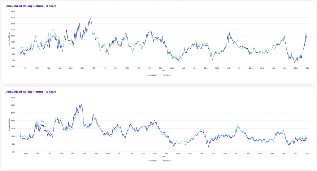
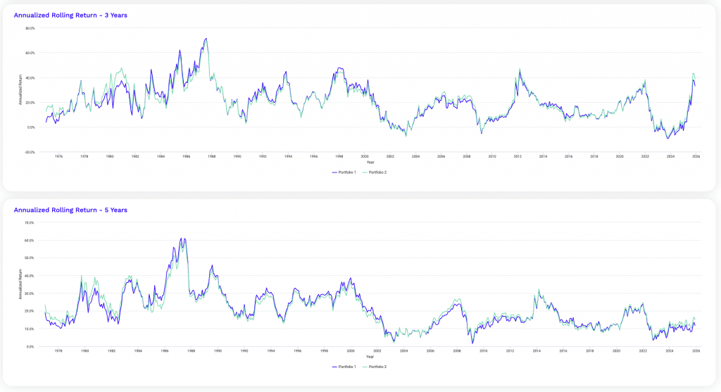
At this leverage level, rolling returns reveal both the strength and the strain of amplified diversification.
Three-year rolling returns show wider dispersion, with extended periods of exceptional performance followed by sharp compressions during tightening cycles and correlation spikes.
Shorter horizons become increasingly sensitive to entry point risk, particularly around inflation-driven regime shifts.
Five-year rolling returns remain smoother and consistently positive, underscoring that diversification still asserts itself over longer horizons.
But recovery slopes flatten compared to lower leverage levels. This means strong rebounds take longer to fully materialize.
The close alignment between portfolios indicates that leverage dominates behavior more than marginal allocation differences.
These charts reinforce that time horizon becomes the decisive variable once leverage reaches this range.
2.5x Leverage
Same allocations:
Portfolio 1
| Asset Class | Allocation |
|---|---|
| US Stock Market | 40.00% |
| 10-year Treasury | 50.00% |
| Gold | 10.00% |
Portfolio 2
| Asset Class | Allocation |
|---|---|
| US Stock Market | 40.00% |
| 10-year Treasury | 45.00% |
| Gold | 15.00% |
Performance Summary
| Metric | Portfolio 1 | Portfolio 2 |
|---|---|---|
| Start Balance | $10,000 | $10,000 |
| End Balance | $58,341,103 | $75,471,854 |
| Annualized Return (CAGR) | 17.45% | 18.01% |
| Standard Deviation | 20.14% | 20.56% |
| Best Year | 75.97% | 76.85% |
| Worst Year | -39.54% | -38.16% |
| Maximum Drawdown | -44.26% | -43.65% |
| Sharpe Ratio | 0.68 | 0.70 |
| Sortino Ratio | 1.09 | 1.12 |
At 2.5x leverage, the portfolios transition fully into a high-octane return profile where compounding power is extraordinary but operational demands are severe.
Ending balances explode to roughly $58 million for Portfolio 1 and over $75 million for Portfolio 2, with annualized returns approaching 18%.
These results start to go beyond what’s realistic for concentrated equity strategies (efficient market and all), yet remain driven by diversified beta rather than single-asset exposure.
Risk, however, goes up sharply.
Volatility moves above 20%, which is less influential than the fact that drawdowns breach the 40% threshold.
Worst-year losses near 40% place pressure on leverage tolerance and investor behavior.
With such drawdowns, behavioral error risks increase.
Risk-adjusted metrics hold up surprisingly well. Sharpe and Sortino ratios edge higher, implying that diversification still contributes meaningfully even as leverage rises.
Portfolio 2 continues to display superior efficiency, delivering higher returns with slightly smaller drawdowns and better downside-adjusted performance.
The defining feature of 2.5x leverage isn’t return potential but survivability.
Only investors with stable financing, strict rebalancing discipline, and the ability to withstand prolonged capital impairment can realistically operate at this level.
The ride is bumpy in order to get these 17-18% CAGRs.
At the same time, 4 out of 5 years are still positive. And in the loss years, most of them are still small. 2022 was an exception was the leveraged beta strategy.
But out key takeaway here is:
For most allocators, this leverage starts getting into an upper bound where the theoretical benefits of diversification collide with real-world constraints on risk tolerance, liquidity, and behavioral endurance.
Risk and Return Metrics
| Metric | Portfolio 1 | Portfolio 2 |
|---|---|---|
| Arithmetic Mean (monthly) | 1.52% | 1.56% |
| Arithmetic Mean (annualized) | 19.81% | 20.48% |
| Geometric Mean (monthly) | 1.35% | 1.39% |
| Geometric Mean (annualized) | 17.45% | 18.01% |
| Standard Deviation (monthly) | 5.81% | 5.93% |
| Standard Deviation (annualized) | 20.14% | 20.56% |
| Downside Deviation (monthly) | 3.43% | 3.49% |
| Maximum Drawdown | -44.26% | -43.65% |
| Benchmark Correlation | 0.81 | 0.79 |
| Beta(*) | 1.04 | 1.04 |
| Alpha (annualized) | 6.12% | 6.72% |
| R2 | 65.43% | 62.50% |
| Sharpe Ratio | 0.68 | 0.70 |
| Sortino Ratio | 1.09 | 1.12 |
| Treynor Ratio (%) | 13.19 | 13.77 |
| Calmar Ratio | 1.67 | 2.01 |
| Modigliani–Modigliani Measure | 15.17% | 15.39% |
| Active Return | 6.57% | 7.14% |
| Tracking Error | 11.86% | 12.60% |
| Information Ratio | 0.55 | 0.57 |
| Skewness | -0.12 | -0.14 |
| Excess Kurtosis | 1.21 | 1.30 |
| Historical Value-at-Risk (5%) | 8.13% | 8.33% |
| Analytical Value-at-Risk (5%) | 8.04% | 8.20% |
| Conditional Value-at-Risk (5%) | 11.30% | 11.28% |
| Upside Capture Ratio (%) | 120.93 | 122.18 |
| Downside Capture Ratio (%) | 94.22 | 93.06 |
| Safe Withdrawal Rate | 10.78% | 13.05% |
| Perpetual Withdrawal Rate | 11.72% | 12.14% |
| Positive Periods | 411 out of 647 (63.52%) | 409 out of 647 (63.21%) |
| Gain/Loss Ratio | 1.13 | 1.15 |
| * US Stock Market is used as the benchmark for calculations. Value-at-risk metrics are monthly values. | ||
The increase in CAGR to roughly 17.5–18.0% reflects a compounding profile where sustained exposure dominates outcomes, and where small differences in allocation efficiency translate into very large terminal wealth gaps over long horizons.
The divergence between Portfolio 1 and Portfolio 2 becomes economically meaningful rather than trivial, with Portfolio 2 finishing more than $17 million ahead from the same starting capital.
Risk metrics show that volatility and drawdowns scale faster than returns beyond this point.
Standard deviation rises into the low 20 percent range, placing these portfolios beyond equity-like volatility despite their diversified construction.
Maximum drawdowns deepen into the mid-40 percent range, which materially alters recovery dynamics. Losses of this magnitude require substantially larger subsequent gains to break even.
This increases reliance on favorable sequencing rather than steady mean reversion.
Calendar-year extremes also widen. Best-year returns exceeding 75% mean that performance becomes highly sensitive to macro alignment, particularly periods of declining real rates or synchronized asset rallies.
Conversely, worst-year losses near 40% imply that adverse market environments are no longer brief interruptions but defining features of the experience.
The dispersion between best and worst outcomes grows large enough that timing, funding stability, rebalancing discipline, and potential behavioral mistakes from the trader/investors exert outsized influence on realized results.
Risk-adjusted measures remain strong.
Sharpe and Sortino ratios suggest that diversification continues to contribute meaningfully to return generation rather than being overwhelmed by leverage.
Nevertheless, these ratios increasingly mask the lived experience of capital volatility.
The trade-off at 2.5x leverage is therefore not efficiency versus inefficiency, but mathematical attractiveness versus practical operability.
The data show that the portfolio still works, but only under conditions where drawdown tolerance, liquidity access, and decision-making discipline are treated as core inputs rather than secondary considerations.
The use of hedges – most notably OTM options and in a way that doesn’t erode long-term returns – becomes more important at this level.
Historical Market Stress Periods
| Stress Period | Start | End | Portfolio 1 | Portfolio 2 |
|---|---|---|---|---|
| Oil Crisis | Oct 1973 | Mar 1974 | -9.09% | -8.43% |
| Black Monday Period | Sep 1987 | Nov 1987 | -30.03% | -29.05% |
| Asian Crisis | Jul 1997 | Jan 1998 | -6.78% | -6.64% |
| Russian Debt Default | Jul 1998 | Oct 1998 | -16.09% | -17.45% |
| Dotcom Crash | Mar 2000 | Oct 2002 | -23.22% | -24.28% |
| Subprime Crisis | Nov 2007 | Mar 2009 | -36.30% | -37.50% |
| COVID-19 Start | Jan 2020 | Mar 2020 | -12.49% | -13.41% |
The stress-period drawdowns at 2.5x leverage show how historical crises translate into materially different capital outcomes once leverage reaches this level.
Losses that were previously manageable now approach thresholds that dominate portfolio behavior for years rather than months.
Black Monday and the subprime crisis produce drawdowns near or above 30%, while the global financial crisis exceeds 36%, pushing recovery requirements into a structurally demanding zone.
Inflation-linked shocks such as the oil crisis and COVID-era volatility also become more consequential, even though their durations are shorter.
Differences between the two portfolios remain incremental.
So, leverage, not allocation nuance, is the primary driver of stress behavior.
These results confirm that at 2.5x leverage, crisis management depends less on diversification mechanics and more on balance sheet strength, funding stability, keeping a clear head, and the capacity to remain fully invested through severe and prolonged dislocations.
Drawdowns for Portfolio 1
| Rank | Start | End | Length | Recovery By | Recovery Time | Underwater Period | Drawdown |
|---|---|---|---|---|---|---|---|
| 1 | Jan 2022 | Sep 2022 | 9 months | Sep 2024 | 2 years | 2 years 9 months | -44.26% |
| 2 | Mar 2008 | Feb 2009 | 1 year | Nov 2009 | 9 months | 1 year 9 months | -36.30% |
| 3 | Mar 1974 | Sep 1974 | 7 months | May 1975 | 8 months | 1 year 3 months | -35.78% |
| 4 | Dec 1980 | Sep 1981 | 10 months | Sep 1982 | 1 year | 1 year 10 months | -30.64% |
| 5 | Sep 1987 | Nov 1987 | 3 months | Apr 1989 | 1 year 5 months | 1 year 8 months | -30.03% |
| 6 | Feb 1980 | Mar 1980 | 2 months | Jun 1980 | 3 months | 5 months | -26.84% |
| 7 | Sep 2000 | Jul 2002 | 1 year 11 months | Sep 2003 | 1 year 2 months | 3 years 1 month | -23.22% |
| 8 | Jul 1983 | May 1984 | 11 months | Oct 1984 | 5 months | 1 year 4 months | -22.77% |
| 9 | Jul 1975 | Sep 1975 | 3 months | Jan 1976 | 4 months | 7 months | -19.27% |
| 10 | Feb 1994 | Nov 1994 | 10 months | Apr 1995 | 5 months | 1 year 3 months | -18.97% |
| Worst 10 drawdowns included above | |||||||
The worst drawdowns for Portfolio 1 at 2.5x leverage show how depth, duration, and recovery interact once leverage dominates the return path.
The 2022 tightening cycle produces the largest impairment, exceeding a 44% loss and remaining underwater for nearly three years.
This episode shows how inflation-driven correlation shifts can overwhelm diversification when leverage is elevated, turning what would otherwise be a cyclical setback into a prolonged capital recovery.
Earlier crises follow a similar pattern.
The global financial crisis and the 1970s inflationary market environment generate drawdowns in the mid-30% range, with recovery times extending well beyond a year despite eventual mean reversion. Notably, recovery speed doesn’t align cleanly with drawdown depth.
Some large losses recover relatively quickly once policy reverses, while others linger due to macro headwinds rather than traditional debt-driven crises.
Short, sharp shocks such as Black Monday still recover faster in absolute time, but the underwater periods remain lengthy because of the magnitude of the initial loss.
The key insight from these data is that leverage converts macro persistence into a dominant risk factor.
At this level, survival depends less on diversification mechanics and more on maintaining exposure through extended periods of discomfort and delayed recovery. There’s more psychological pressure.
Drawdowns for Portfolio 2
| Rank | Start | End | Length | Recovery By | Recovery Time | Underwater Period | Drawdown |
|---|---|---|---|---|---|---|---|
| 1 | Jan 2022 | Sep 2022 | 9 months | Aug 2024 | 1 year 11 months | 2 years 8 months | -43.65% |
| 2 | Mar 2008 | Feb 2009 | 1 year | Nov 2009 | 9 months | 1 year 9 months | -37.50% |
| 3 | Mar 1974 | Sep 1974 | 7 months | May 1975 | 8 months | 1 year 3 months | -35.93% |
| 4 | Dec 1980 | Sep 1981 | 10 months | Oct 1982 | 1 year 1 month | 1 year 11 months | -33.25% |
| 5 | Feb 1980 | Mar 1980 | 2 months | Jun 1980 | 3 months | 5 months | -29.25% |
| 6 | Sep 1987 | Nov 1987 | 3 months | May 1989 | 1 year 6 months | 1 year 9 months | -29.05% |
| 7 | Sep 2000 | Jul 2002 | 1 year 11 months | Sep 2003 | 1 year 2 months | 3 years 1 month | -24.28% |
| 8 | Jul 1983 | May 1984 | 11 months | Jan 1985 | 8 months | 1 year 7 months | -22.74% |
| 9 | Jul 1975 | Sep 1975 | 3 months | Jan 1976 | 4 months | 7 months | -20.52% |
| 10 | Feb 1994 | Nov 1994 | 10 months | Apr 1995 | 5 months | 1 year 3 months | -17.75% |
| Worst 10 drawdowns included above | |||||||
3x Leverage
Same allocation at 3x:
Portfolio 1
| Asset Class | Allocation |
|---|---|
| US Stock Market | 40.00% |
| 10-year Treasury | 50.00% |
| Gold | 10.00% |
Portfolio 2
| Asset Class | Allocation |
|---|---|
| US Stock Market | 40.00% |
| 10-year Treasury | 45.00% |
| Gold | 15.00% |
Performance Summary
| Metric | Portfolio 1 | Portfolio 2 |
|---|---|---|
| Start Balance | $10,000 | $10,000 |
| End Balance | $183,021,018 | $246,273,957 |
| Annualized Return (CAGR) | 19.97% | 20.63% |
| Standard Deviation | 24.16% | 24.67% |
| Best Year | 93.26% | 94.59% |
| Worst Year | -46.49% | -44.99% |
| Maximum Drawdown | -51.28% | -50.62% |
| Sharpe Ratio | 0.70 | 0.71 |
| Sortino Ratio | 1.11 | 1.14 |
At 3x leverage, compounding accelerates dramatically, with ending balances exceeding $183 million for Portfolio 1 and $246 million for Portfolio 2 from the same $10,000 starting capital.
Annualized returns approach or exceed 20%, placing these results among the highest sustained long-term returns achievable through systematic exposure rather than concentrated bets.
Risk expands accordingly.
Volatility rises into the mid-20 percent range, and maximum drawdowns exceed 50%.
At this depth, losses are no longer episodic setbacks but defining events that dominate portfolio psychology, funding requirements, and rebalancing feasibility.
Worst calendar-year losses near 45% imply that multi-year recoveries are not just possible but likely, especially when adverse macro regimes persist.
Funding costs are 6% per year, due the extra two turns of leverage at 3%.
Despite this, risk-adjusted metrics remain surprisingly stable.
Sharpe and Sortino ratios improve slightly, so diversification continues to generate excess return even at this leverage.
Portfolio 2 again demonstrates marginally better efficiency. You get higher returns with slightly smaller drawdowns and stronger downside-adjusted performance.
The central lesson of 3x leverage isn’t about return potential, which is indisputable, but about feasibility.
This level assumes uninterrupted access to low-cost leverage, strict risk controls, and an investor or trader capable of enduring prolonged drawdowns without forced deleveraging.
The data show that the portfolio still functions statistically, but survival becomes the primary constraint.
Risk and Return Metrics
| Metric | Portfolio 1 | Portfolio 2 |
|---|---|---|
| Arithmetic Mean (monthly) | 1.77% | 1.83% |
| Arithmetic Mean (annualized) | 23.44% | 24.28% |
| Geometric Mean (monthly) | 1.53% | 1.58% |
| Geometric Mean (annualized) | 19.97% | 20.63% |
| Standard Deviation (monthly) | 6.98% | 7.12% |
| Standard Deviation (annualized) | 24.16% | 24.67% |
| Downside Deviation (monthly) | 4.14% | 4.21% |
| Maximum Drawdown | -51.28% | -50.62% |
| Benchmark Correlation | 0.81 | 0.79 |
| Beta(*) | 1.25 | 1.25 |
| Alpha (annualized) | 6.74% | 7.46% |
| R2 | 65.43% | 62.50% |
| Sharpe Ratio | 0.70 | 0.71 |
| Sortino Ratio | 1.11 | 1.14 |
| Treynor Ratio (%) | 13.42 | 14.00 |
| Calmar Ratio | 1.64 | 2.00 |
| Modigliani–Modigliani Measure | 15.36% | 15.57% |
| Active Return | 9.09% | 9.75% |
| Tracking Error | 14.74% | 15.59% |
| Information Ratio | 0.62 | 0.63 |
| Skewness | -0.12 | -0.14 |
| Excess Kurtosis | 1.21 | 1.30 |
| Historical Value-at-Risk (5%) | 9.80% | 10.04% |
| Analytical Value-at-Risk (5%) | 9.70% | 9.88% |
| Conditional Value-at-Risk (5%) | 13.61% | 13.59% |
| Upside Capture Ratio (%) | 146.85 | 148.39 |
| Downside Capture Ratio (%) | 113.85 | 112.56 |
| Safe Withdrawal Rate | 12.37% | 15.47% |
| Perpetual Withdrawal Rate | 13.60% | 14.08% |
| Positive Periods | 407 out of 647 (62.91%) | 409 out of 647 (63.21%) |
| Gain/Loss Ratio | 1.14 | 1.13 |
| * US Stock Market is used as the benchmark for calculations. Value-at-risk metrics are monthly values. | ||
At 3x leverage, the detailed risk and return metrics show a portfolio that’s no longer defined by moderation but by exposure intensity and sequencing sensitivity.
Monthly volatility rises to nearly 7%, which is around half of the annual stock market volatility in just one month.
That materially increases the dispersion of outcomes even though long-term compounding remains strong.
The widening gap between arithmetic and geometric returns reflects a higher volatility tax, yet the drag doesn’t overwhelm growth. So, the diversification is still functioning rather than collapsing.
Equity linkage becomes more pronounced. Beta rises above 1.2, and upside capture exceeds 145%, meaning the portfolio now participates more aggressively than the equity market during strong expansions.
At the same time, downside capture also exceeds 110%, confirming that drawdowns are no longer meaningfully cushioned during equity-led selloffs.
This is reinforced by higher value-at-risk and conditional value-at-risk figures, which place short-horizon losses firmly into territory that demands large liquidity buffers.
Several efficiency measures remain favorable. Alpha continues to expand (though we covered earlier in the article why this isn’t true alpha in the genuine sense), and information ratios improve. This implies that excess returns relative to the benchmark are becoming more consistent rather than sporadic.
The Modigliani-Modigliani measure also rises. This means that on a volatility-adjusted basis, returns remain competitive despite the elevated risk profile.
However, Calmar ratios flatten and tail metrics worsen. Drawdown depth is increasingly dictating capital recovery rather than return generation.
Withdrawal rates climb sharply, but these figures assume uninterrupted exposure and ignore the behavioral stress imposed by 50% drawdowns, so you can’t read too much into them.
The trade-off at this level is clear. The portfolio remains statistically attractive, but the margin for operational error narrows dramatically.
The leverage outweighs allocation design itself.

Historical Market Stress Periods
| Stress Period | Start | End | Portfolio 1 | Portfolio 2 |
|---|---|---|---|---|
| Oil Crisis | Oct 1973 | Mar 1974 | -10.96% | -10.17% |
| Black Monday Period | Sep 1987 | Nov 1987 | -35.50% | -34.41% |
| Asian Crisis | Jul 1997 | Jan 1998 | -8.19% | -8.02% |
| Russian Debt Default | Jul 1998 | Oct 1998 | -19.30% | -20.90% |
| Dotcom Crash | Mar 2000 | Oct 2002 | -28.30% | -29.51% |
| Subprime Crisis | Nov 2007 | Mar 2009 | -43.10% | -44.46% |
| COVID-19 Start | Jan 2020 | Mar 2020 | -14.99% | -16.08% |
The stress-period outcomes at 3x leverage illustrate how historical crises translate into materially different portfolio experiences once amplification reaches this level.
Losses during major shocks consistently move into ranges that dominate long-term capital trajectories rather than appearing as temporary interruptions.
Events that were previously uncomfortable become defining episodes requiring years of recovery.
Equity-driven shocks stand out most clearly.
Black Monday and the dotcom crash now produce drawdowns approaching or exceeding 30 percent, while the subprime crisis drives losses above 40 percent.
At this depth, recovery depends heavily on policy response timing and macro regime shifts rather than simple market normalization.
The portfolio’s path forward becomes contingent on remaining solvent and invested through extended periods of adverse market environments.
Inflation-related stress also becomes more impactful.
The oil crisis and COVID shock generate losses near 10-15%.
Region-specific crises, such as the Asian crisis and Russian debt default, remain less damaging but still produce double-digit drawdowns. Leverage magnifies even contained shocks.
Differences between the two portfolios remain secondary.
Portfolio 2 generally shows slightly smaller losses during inflationary and liquidity-driven events, while Portfolio 1 marginally outperforms in some deflationary drawdowns.
But these distinctions are overshadowed by the leverage effect itself, which drives the dominant behavior.
The broader implication is that at 3x leverage, historical stress periods cease to be normal analytical checkpoints and instead become operational stress tests.
Survival depends on the ability to endure prolonged capital impairment without forced deleveraging.
Drawdowns for Portfolio 1
| Rank | Start | End | Length | Recovery By | Recovery Time | Underwater Period | Drawdown |
|---|---|---|---|---|---|---|---|
| 1 | Jan 2022 | Sep 2022 | 9 months | May 2025 | 2 years 8 months | 3 years 5 months | -51.28% |
| 2 | Mar 2008 | Feb 2009 | 1 year | Apr 2010 | 1 year 2 months | 2 years 2 months | -43.10% |
| 3 | Mar 1974 | Sep 1974 | 7 months | May 1975 | 8 months | 1 year 3 months | -41.67% |
| 4 | Dec 1980 | Sep 1981 | 10 months | Sep 1982 | 1 year | 1 year 10 months | -36.25% |
| 5 | Sep 1987 | Nov 1987 | 3 months | May 1989 | 1 year 6 months | 1 year 9 months | -35.50% |
| 6 | Feb 1980 | Mar 1980 | 2 months | Jun 1980 | 3 months | 5 months | -31.84% |
| 7 | Sep 2000 | Jul 2002 | 1 year 11 months | Oct 2003 | 1 year 3 months | 3 years 2 months | -28.30% |
| 8 | Jul 1983 | May 1984 | 11 months | Nov 1984 | 6 months | 1 year 5 months | -27.38% |
| 9 | Jul 1975 | Sep 1975 | 3 months | Jan 1976 | 4 months | 7 months | -22.95% |
| 10 | Feb 1994 | Nov 1994 | 10 months | May 1995 | 6 months | 1 year 4 months | -22.93% |
| Worst 10 drawdowns included above | |||||||
Drawdowns for Portfolio 2
| Rank | Start | End | Length | Recovery By | Recovery Time | Underwater Period | Drawdown |
|---|---|---|---|---|---|---|---|
| 1 | Jan 2022 | Sep 2022 | 9 months | Sep 2024 | 2 years | 2 years 9 months | -50.62% |
| 2 | Mar 2008 | Feb 2009 | 1 year | Apr 2010 | 1 year 2 months | 2 years 2 months | -44.46% |
| 3 | Mar 1974 | Sep 1974 | 7 months | May 1975 | 8 months | 1 year 3 months | -41.85% |
| 4 | Dec 1980 | Sep 1981 | 10 months | Oct 1982 | 1 year 1 month | 1 year 11 months | -39.15% |
| 5 | Feb 1980 | Mar 1980 | 2 months | Jun 1980 | 3 months | 5 months | -34.69% |
| 6 | Sep 1987 | Nov 1987 | 3 months | May 1989 | 1 year 6 months | 1 year 9 months | -34.41% |
| 7 | Sep 2000 | Jul 2002 | 1 year 11 months | Oct 2003 | 1 year 3 months | 3 years 2 months | -29.51% |
| 8 | Jul 1983 | May 1984 | 11 months | Jan 1985 | 8 months | 1 year 7 months | -27.32% |
| 9 | Jul 1975 | Sep 1975 | 3 months | Feb 1976 | 5 months | 8 months | -24.40% |
| 10 | Feb 1994 | Nov 1994 | 10 months | Apr 1995 | 5 months | 1 year 3 months | -21.51% |
| Worst 10 drawdowns included above | |||||||
The worst drawdown tables at 3x leverage make clear that portfolio outcomes are dominated less by frequency of losses and more by depth and recovery burden.
The largest drawdowns cluster around the same macro regimes seen at lower leverage, but their magnitude and persistence expand sharply.
The 2022 inflation and tightening cycle becomes the defining event, producing drawdowns slightly above 50 percent for both portfolios and underwater periods approaching three and a half years. This is a prolonged impairment that reshapes capital trajectories.
Earlier systemic crises show similar amplification. The global financial crisis generates drawdowns in the low-to-mid 40 percent range, with recoveries taking more than a year after the trough and over two years spent underwater.
The 1970s inflation shock produces comparable depth. Elongated adverse macro regimes, rather than sudden crashes, drive the most punishing outcomes under leverage. In contrast, shorter shocks such as Black Monday still recover faster in calendar time, but the sheer depth of the initial loss extends underwater periods well beyond the event itself.
A key observation is that recovery time doesn’t scale proportionally with drawdown size. Some large losses recover relatively quickly once policy or valuation conditions reverse, while others linger due to structural headwinds.
This introduces a heavy dependence on regime sequencing rather than simple mean reversion.
Differences between Portfolio 1 and Portfolio 2 remain consistent but secondary. Portfolio 2 generally experiences marginally smaller peak drawdowns and slightly faster recoveries in inflation-sensitive episodes, while Portfolio 1 shows similar behavior in deflationary or liquidity-driven shocks. But as mentioned, these distinctions are overwhelmed by leverage effects.
At this level, the dominant risk is endurance.
The use of cost-effective hedges like options starts becoming important at this 2.5x-3x+ level.
Rolling Returns
| Roll Period | Portfolio 1 | Portfolio 2 | ||||
|---|---|---|---|---|---|---|
| Average | High | Low | Average | High | Low | |
| 1 year | 22.81% | 186.87% | -46.70% | 23.33% | 185.03% | -45.89% |
| 3 years | 20.23% | 71.55% | -9.28% | 20.40% | 70.24% | -8.30% |
| 5 years | 20.46% | 61.11% | 1.48% | 20.51% | 58.80% | 1.94% |
| 7 years | 20.61% | 45.56% | 5.71% | 20.59% | 43.13% | 6.51% |
| 10 years | 20.77% | 37.57% | 5.64% | 20.56% | 36.74% | 6.38% |
| 15 years | 20.87% | 34.76% | 9.81% | 20.60% | 32.90% | 9.99% |
The rolling return analysis provides the clearest picture of how leveraged diversification behaves across time horizons, independent of any single start or end date.
At short horizons, outcomes are highly dispersed but variance dominates at small time horizons.
Year to year returns show extreme variability, with averages in the low-20% range but highs exceeding 180 percent and lows approaching minus 45 percent.
So, short-term results are dominated by sequencing rather than structural return characteristics. At this leverage level, entry point risk is decisive over short windows.
As the horizon extends, dispersion compresses meaningfully. Three-year rolling returns still display volatility, but the range narrows substantially. Negative outcomes remain possible, yet they are far less severe than at the one-year level.
Five-year rolling returns mark a critical transition. The worst outcomes turn positive, and the spread between high and low contracts further. Leverage risk becomes increasingly manageable as time horizon lengthens.
From seven years onward, consistency dominates. Average rolling returns stabilize near 20% across both portfolios, while the minimum outcomes rise steadily into mid-single digits.
By ten and fifteen years, the return bands tighten a lot. The difference between best and worst outcomes shrinks to levels that are small relative to the overall return magnitude. Long-horizon investors become more insulated from timing risk and can even use the equity gains to modestly de-lever as time goes on if they wish.
The charts reinforce this numerically.
Three-year rolling returns oscillate widely during regime transitions, particularly inflationary tightening and post-bubble periods.
Five-year returns are smoother, with drawdowns appearing as shallow valleys rather than deep troughs. Horizon length is the dominant driver of realized outcomes.
3x Leverage (But Changing the Portfolio)
Okay, we’ve pretty well established the risks associated with the 3x portfolio associated with our allocations above.
You can do those, but you don’t know the future exactly and sequencing risk is so high.
So, let’s go easier on the equities and keep gold the same or slightly higher.
Portfolio 1
| Asset Class | Allocation |
|---|---|
| US Stock Market | 25.00% |
| 10-year Treasury | 60.00% |
| Gold | 15.00% |
Portfolio 2
| Asset Class | Allocation |
|---|---|
| US Stock Market | 25.00% |
| 10-year Treasury | 55.00% |
| Gold | 20.00% |
Performance Summary
| Metric | Portfolio 1 | Portfolio 2 |
|---|---|---|
| Start Balance | $10,000 | $10,000 |
| End Balance | $97,582,700 | $125,647,144 |
| Annualized Return (CAGR) | 18.57% | 19.13% |
| Standard Deviation | 22.05% | 22.92% |
| Best Year | 100.86% | 106.75% |
| Worst Year | -42.93% | -41.39% |
| Maximum Drawdown | -47.94% | -47.12% |
| Sharpe Ratio | 0.69 | 0.69 |
| Sortino Ratio | 1.14 | 1.15 |
At 3x leverage, shifting the portfolio mix toward heavier Treasury and gold exposure meaningfully alters the risk profile without eliminating the core leverage effects.
Both portfolios still deliver exceptional compounding.
Annualized returns remain near 19 percent, only modestly below the more equity-heavy configurations.
Volatility declines slightly relative to the prior 3x configurations, settling in the low-20% range.
Best-year returns exceed 100 percent, cso leverage still produces extreme upside during favorable macro regimes.
At the same time, worst-year losses and maximum drawdowns remain severe, clustering in the low-to-mid/mid-high 40% range. These levels materially shape recovery requirements and trader/investor experience.
Risk-adjusted metrics flatten. Sharpe ratios no longer improve with added defensive assets. So there’s diminishing marginal benefits from further smoothing at this leverage level.
Portfolio 2’s higher gold allocation delivers slightly better outcomes.
So gold has a quality role in reducing drawdown depth rather than boosting average returns.
Overall, these allocations show that composition can moderate volatility at 3x leverage, but can’t fundamentally change the endurance demands imposed by such amplification.
Risk and Return Metrics
| Metric | Portfolio 1 | Portfolio 2 |
|---|---|---|
| Arithmetic Mean (monthly) | 1.63% | 1.68% |
| Arithmetic Mean (annualized) | 21.40% | 22.20% |
| Geometric Mean (monthly) | 1.43% | 1.47% |
| Geometric Mean (annualized) | 18.57% | 19.13% |
| Standard Deviation (monthly) | 6.37% | 6.62% |
| Standard Deviation (annualized) | 22.05% | 22.92% |
| Downside Deviation (monthly) | 3.61% | 3.73% |
| Maximum Drawdown | -47.94% | -47.12% |
| Benchmark Correlation | 0.58 | 0.56 |
| Beta(*) | 0.82 | 0.82 |
| Alpha (annualized) | 10.01% | 10.70% |
| R2 | 33.97% | 31.28% |
| Sharpe Ratio | 0.69 | 0.69 |
| Sortino Ratio | 1.14 | 1.15 |
| Treynor Ratio (%) | 18.35 | 19.21 |
| Calmar Ratio | 1.69 | 2.09 |
| Modigliani–Modigliani Measure | 15.21% | 15.25% |
| Active Return | 7.70% | 8.26% |
| Tracking Error | 18.13% | 19.21% |
| Information Ratio | 0.42 | 0.43 |
| Skewness | 0.14 | 0.16 |
| Excess Kurtosis | 1.27 | 1.34 |
| Historical Value-at-Risk (5%) | 8.19% | 8.70% |
| Analytical Value-at-Risk (5%) | 8.84% | 9.20% |
| Conditional Value-at-Risk (5%) | 11.83% | 12.12% |
| Upside Capture Ratio (%) | 104.42 | 105.70 |
| Downside Capture Ratio (%) | 66.58 | 65.51 |
| Safe Withdrawal Rate | 15.36% | 18.64% |
| Perpetual Withdrawal Rate | 12.57% | 12.99% |
| Positive Periods | 400 out of 647 (61.82%) | 393 out of 647 (60.74%) |
| Gain/Loss Ratio | 1.20 | 1.26 |
| * US Stock Market is used as the benchmark for calculations. Value-at-risk metrics are monthly values. | ||
These statistics show how the higher Treasury and gold weights reshape portfolio behavior at 3x leverage in a more structural way than earlier configurations.
Most notable is the reduced linkage to the equity benchmark.
Correlation falls into the mid-0.5 range and R² drops to roughly one-third. So, returns are being driven far less by equity beta and far more by cross-asset dynamics amplified through leverage. Beta remains below 0.85 despite 3x exposure.
Return quality remains strong. Geometric returns stay close to arithmetic returns, which means that volatility drag, while present, hasn’t overwhelmed compounding.
Alpha expands meaningfully into double digits, which suggests that leverage is magnifying diversified factor premia rather than simply increasing basic market exposure.
Information ratios remain positive, which means that excess returns are relatively stable rather than episodic.
Risk characteristics show a clearer trade-off.
Volatility stabilizes near the low-20% range, slightly lower than more equity-heavy 3x portfolios, while downside deviation and drawdown metrics show modest improvement.
Maximum drawdowns remain severe but don’t worsen relative to prior 3x configurations. The added defensive exposure helps limit tail depth without eliminating it.
Value-at-risk and conditional value-at-risk measures remain high, but their increase is controlled.
Capture ratios show a meaningful asymmetry. Upside capture is near parity with equities, while downside capture remains well below 70 percent.
This means that the portfolio still gives up less in market declines than it gains in advances, even under high leverage.
Calmar ratios improve notably for Portfolio 2, because of the better drawdown efficiency.
Sustainability metrics look good. Safe and perpetual withdrawal rates rise a lot. So for investors with stable leverage financing and long horizons, income durability improves despite higher volatility.
Overall, these results show that asset composition becomes more important at higher leverage. Not to boost returns, but to control correlation structure, tail behavior, recovery efficiency, and to make the portfolio easier to deal with for traders/investors managing it.
Historical Market Stress Periods
| Stress Period | Start | End | Portfolio 1 | Portfolio 2 |
|---|---|---|---|---|
| Oil Crisis | Oct 1973 | Mar 1974 | -5.08% | -4.45% |
| Black Monday Period | Sep 1987 | Nov 1987 | -20.41% | -19.27% |
| Asian Crisis | Jul 1997 | Jan 1998 | -7.10% | -6.92% |
| Russian Debt Default | Jul 1998 | Oct 1998 | -11.29% | -12.94% |
| Dotcom Crash | Mar 2000 | Oct 2002 | -9.52% | -11.33% |
| Subprime Crisis | Nov 2007 | Mar 2009 | -33.75% | -36.97% |
| COVID-19 Start | Jan 2020 | Mar 2020 | -4.24% | -5.37% |
Losses during inflationary and liquidity-driven shocks are materially reduced compared to equity-heavier 3x portfolios.
The oil crisis, Asian crisis, and COVID shock remain contained to mid-single-digit drawdowns.
Even Black Monday produces losses closer to 20% rather than the mid-30% range seen previously at 3x leverage.
Nonetheless, extended equity bear markets still impose high costs.
The dotcom and subprime crises remain the dominant stress events, with drawdowns approaching or exceeding 30%.
Differences between Portfolio 1 and Portfolio 2 remain modest, though Portfolio 2’s higher gold allocation slightly improves inflation-/currency-related outcomes.
Overall, the data show that defensive composition can materially reduce stress severity at this kind of leverage.
Drawdowns for Portfolio 1
| Rank | Start | End | Length | Recovery By | Recovery Time | Underwater Period | Drawdown |
|---|---|---|---|---|---|---|---|
| 1 | Sep 2021 | Sep 2022 | 1 year 1 month | Jun 2025 | 2 years 9 months | 3 years 10 months | -47.94% |
| 2 | Jul 1980 | Sep 1981 | 1 year 3 months | Sep 1982 | 1 year | 2 years 3 months | -38.26% |
| 3 | Mar 2008 | Oct 2008 | 8 months | Nov 2009 | 1 year 1 month | 1 year 9 months | -33.75% |
| 4 | Feb 1980 | Mar 1980 | 2 months | Jun 1980 | 3 months | 5 months | -32.44% |
| 5 | Mar 1974 | Sep 1974 | 7 months | Feb 1975 | 5 months | 1 year | -31.48% |
| 6 | May 1983 | May 1984 | 1 year 1 month | Nov 1984 | 6 months | 1 year 7 months | -26.93% |
| 7 | Feb 1994 | Nov 1994 | 10 months | May 1995 | 6 months | 1 year 4 months | -23.39% |
| 8 | Aug 1987 | Nov 1987 | 4 months | Apr 1989 | 1 year 5 months | 1 year 9 months | -20.74% |
| 9 | Jul 1975 | Sep 1975 | 3 months | Feb 1976 | 5 months | 8 months | -20.04% |
| 10 | Oct 1979 | Oct 1979 | 1 month | Dec 1979 | 2 months | 3 months | -19.51% |
| Worst 10 drawdowns included above | |||||||
Drawdowns for Portfolio 2
| Rank | Start | End | Length | Recovery By | Recovery Time | Underwater Period | Drawdown |
|---|---|---|---|---|---|---|---|
| 1 | Sep 2021 | Sep 2022 | 1 year 1 month | Feb 2025 | 2 years 5 months | 3 years 6 months | -47.12% |
| 2 | Jul 1980 | Sep 1981 | 1 year 3 months | Oct 1982 | 1 year 1 month | 2 years 4 months | -40.81% |
| 3 | Mar 2008 | Oct 2008 | 8 months | Nov 2009 | 1 year 1 month | 1 year 9 months | -36.97% |
| 4 | Feb 1980 | Mar 1980 | 2 months | Jun 1980 | 3 months | 5 months | -35.19% |
| 5 | Mar 1974 | Sep 1974 | 7 months | Feb 1975 | 5 months | 1 year | -31.94% |
| 6 | May 1983 | May 1984 | 1 year 1 month | Jan 1985 | 8 months | 1 year 9 months | -26.97% |
| 7 | Oct 2012 | Jun 2013 | 9 months | Jan 2015 | 1 year 7 months | 2 years 4 months | -22.24% |
| 8 | Feb 1994 | Nov 1994 | 10 months | May 1995 | 6 months | 1 year 4 months | -21.98% |
| 9 | Jul 1975 | Sep 1975 | 3 months | Mar 1976 | 6 months | 9 months | -21.62% |
| 10 | Aug 1987 | Nov 1987 | 4 months | Apr 1989 | 1 year 5 months | 1 year 9 months | -19.71% |
| Worst 10 drawdowns included above | |||||||
The 2021-2022 tightening cycle dominates for both portfolios. That produced drawdowns just under 48% and underwater periods stretching well beyond three years.
This shows that inflation-driven correlation shifts remain the most challenging environment for these portfolios, regardless of asset mix. This is because both the stocks and bonds portion correlate together and the gold isn’t enough of an offset.
Earlier inflationary episodes from the late 1970s and early 1980s also feature prominently.
These drawdowns are deep but recover more quickly once policy reverses. In contrast, the 2008 global financial crisis produces slightly smaller drawdowns than the inflationary episodes – because bonds were a good offset in this growth-driven disinflationary event – but still imposes extended underwater periods due to slow balance sheet repair and weak growth.
Short, violent shocks behave differently. Events like 1987 produce drawdowns near 20% with relatively fast recoveries in absolute time, though underwater periods still extend well beyond a year because leverage magnifies the initial loss.
Notably, Portfolio 2 consistently shows slightly smaller peak drawdowns and marginally shorter recovery paths in the largest events. This shows the stabilizing influence of higher gold exposure.
The broader pattern is that leverage can magnify persistence risk just as it can magnify shock risk.
Drawdowns become multi-year experiences not because markets fail to recover, but because the capital base has to climb out of much deeper troughs.
Accordingly, tail risk protection becomes more important – and figuring out how to do it cost-effectively so it’s not too much of a drag on long-term performance.
How to Generate Leverage
So, how do you generate leverage in a portfolio?
Let’s look at the options.
Retail vs. Institutional Leverage
Most important is the cost of leverage.
For a 1-year holding, your benchmark borrowing cost is going to be the 1-year SOFR.
So, if you leverage your portfolio with any margin loan, option, future, and so on, you’re looking to pay around that rate.
Of course, that’s before the markup. And with retail brokers that can add several percent on top. If your margin loan rate is 7%+, when risk-free rates are well below that, you can’t reasonably lever using those rates.
If you have no other source of reasonable funding, consider options and futures.
They have embedded leverage (e.g., contango costs in futures) that’s closer to what you see for institutional levels.
Those who are able to borrow and lend at fair value are active in these markets and these benefits also transfer downstream to retail traders who also operate in these markets.
Using Options for Leverage
Options are a type of derivative that provides a risk-limited way to achieve leverage in your portfolio.
They provide the right, but not the obligation, to buy or sell an underlying asset at a predetermined price within a specific period.
When you buy an option, you control a larger amount of the underlying asset for a fraction of its direct purchase cost.
For example, buying a call option allows a trader to benefit from a rise in the underlying asset’s price with a much smaller initial outlay than buying the asset outright.
Conversely, buying put options can protect an investor from a decline in the asset’s value.
However, options can expire worthless if they’re out-of-the-money at expiry, leading to a total loss of the initial investment.
The complex nature of options, along with their time sensitivity (expiration dates), requires a nuanced understanding of the market.
Deep ITM Call Options
Often the best way for retail traders to leverage their portfolios is by buying deep in-the-money call options.
You still pay the tail risk but with close to institutional borrowing costs.
For example, let’s say SPY is $683.64 per share. If you choose a $450 strike, that’s $233.64 per share of “moneyness.”
With 100 shares per contract, that’s $23,364.
The premium for the option is $25,566.
Let’s say $25,570 after transaction costs.
To figure out the transaction costs, we subtract the difference, then divide by the spot price.
So that’s $25,570 – $23,364 = $2,206
$2,206 / $68,364 = 3.22% (The $68,364 comes from multiplying the per share price by 100, given 100 shares per contract.)
That beats the high single-digit rates that would be common at retail markups.
And you’re controlling over $68,000 worth of assets for a cash outlay of $25,570, for a leverage ratio of 2.67x.
Leverage through Futures
Like options, futures contracts offer another way to achieve leverage in a portfolio.
They’re agreements to buy or sell an asset at a future date for a specified price.
In futures trading, the trader only needs to have a small fraction of the total contract value available, known as the margin.
This allows for large positions to be taken with a relatively small amount of capital. This effectively creates leverage.
Traders nonetheless need to watch out for implied costs, such as contango, that can effectively be like paying interest.
Futures
If we look at futures, we can look at the costs over one year.
The front month:
The one-year future:
Dividing the two, we take $708,877 / $688,350 = 2.98%