Quadratic Programming in Trading & Investing (Coding Example)

Quadratic programming (QP) is a type of mathematical optimization used in portfolio management and trading/investment strategies.

Its primary function is to optimize asset allocation to achieve the best possible risk-adjusted returns.

Key Takeaways – Quadratic Programming

• Optimizes Portfolio Allocation – Quadratic programming helps determine the optimal asset mix to maximize returns for a given risk level.
• Manages Risk Effectively – It helps in minimizing portfolio risk by calculating the variance-covariance matrix for asset returns, which allows for more precise risk management strategies.
• Enhances Diversification – Quadratic programming aids in identifying non-obvious asset allocation strategies that improve portfolio diversification and reduce volatility.
• Coding Example – We have a coding example of quadratic programming later in the article.

Understanding Quadratic Programming

Quadratic programming involves the minimization or maximization of a quadratic function subject to linear constraints.

In the context of trading and investing:

• the quadratic function typically represents the portfolio’s variance (or risk), and
• the linear constraints can reflect budget limitations, risk exposure caps, or other investment guidelines

Math Behind Quadratic Programming

Here is a basic overview of quadratic programming for portfolio optimization:

The optimization problem is to maximize portfolio return while minimizing risk:

• Maximize: Rp = wTμ
• Minimize: Vp = wT Σ w
• Subject to: Σ wi = 1 (fully invested) L ≤ wi ≤ U (asset weight bounds)

Where:

• w = Vector of asset weights in portfolio
• μ = Vector of expected asset returns
• Σ = Covariance matrix of asset returns
• Rp = Return of portfolio
• Vp = Variance (risk) of portfolio
• L, U = Lower and upper limits on assets

This forms a quadratic programming problem with a quadratic objective function (portfolio variance) and linear constraints (budget, bounds).

The optimal asset weights w* are obtained by solving:

Minimize: (1/2)wT Σ w (Subject to linear constraints)

Quadratic programming uses iterative numerical methods like active set or interior point to solve for the optimum asset allocations.

The result is the portfolio on the “efficient frontier” – i.e., the highest return for a given risk level that satisfies the constraints (covered more below).

The quadratic form allows incorporating covariance between assets and the impact of diversification.

Applications in Portfolio Optimization

Risk Minimization

Quadratic programming is used in mean-variance analysis, a framework introduced by Harry Markowitz in 1952.

Traders use QP to construct a portfolio that offers the highest expected return for a given level of risk.

Or alternatively, the lowest risk for a given level of expected return.

By solving a QP problem, traders can identify the asset weights that’ll minimize the portfolio’s overall variance.

Asset Allocation

Traders also use quadratic programming to allocate assets in a way that aligns with their risk tolerance and goals.

This involves balancing the trade-off between risk and return, ensuring diversification, and adhering to the constraints of their strategy.

Benefits in Trading & Investing

Efficient Frontier Identification

Quadratic programming enables traders to locate the efficient frontier, a set of optimal portfolios that offer the highest expected return for a given level of risk.

Graphically, the efficient frontier looks like this, where the dark blue part of the graph (in this case) is considered the optimal allocation.

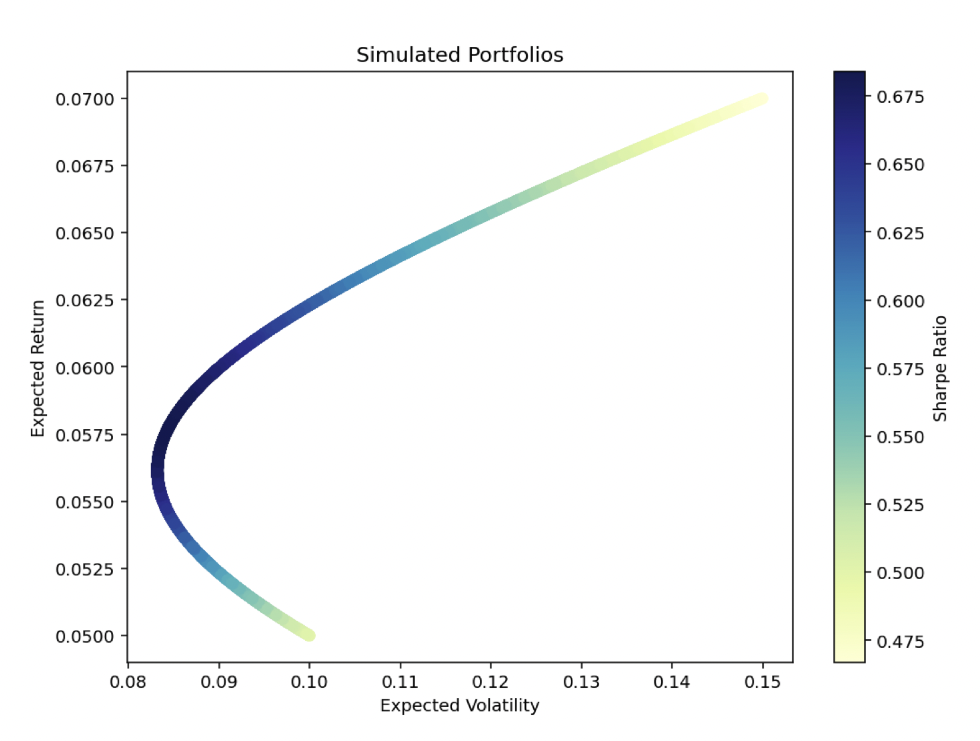
This identification is important for strategic asset allocation and helps traders make decisions based on their risk appetite.

Customization of Trading/Investment Strategies

QP allows for the customization of trading/investment strategies by incorporating various constraints, such as limitations on short-selling, asset- or sector-specific caps, or minimum investment requirements.

This flexibility ensures that the optimized portfolio aligns with individual preferences and regulatory requirements.

Challenges, Criticisms & Considerations

Model Assumptions

Quadratic programming relies on certain assumptions, including the normal distribution of returns and the stability of covariances over time.

Traders must be aware of these assumptions and consider their implications on the model’s predictive accuracy.

Computational Complexity

Solving large-scale quadratic programming problems can be computationally intensive.

It’s most true when dealing with vast asset universes or complex constraint structures.

Efficient algorithms and high-performance computing resources are important to address these challenges.

Lack of Dimensionality

The mean-variance framework often doesn’t take into consideration the high level of dimensionality inherent in financial data and the optimization process.

For this reason, modern quantitative finance is increasingly trending toward more sophisticated geometric approaches that take into account dimensionality, like those covered in the articles below:

Related

• Differential Geometry
• Symplectic Geometry
• Riemannian Manifolds
• Manifold Learning
• Differential Topology
• Geometric Mechanics
• Complex Analysis in Markets
• Tensor Theory in Markets

Critical Line Method

The Critical Line Method is an algorithmic approach used in portfolio optimization (notably for solving the mean-variance optimization problem formulated by Harry Markowitz).

This method efficiently identifies the optimal asset allocation that maximizes return for a given level of risk or minimizes risk for a given level of return.

It operates by constructing the efficient frontier, a set of optimal portfolios, through linear and quadratic programming.

The Critical Line Method stands out for its precision in handling the complexities of real-world constraints, such as buy-in thresholds, asset bounds, and transaction costs.

Its stepwise, systematic process navigates through these constraints, adjusting asset weights to find the most efficient portfolios.

This method remains fundamental in modern portfolio theory by helping make more data-driven, strategic allocation decisions.

Quadratic Programming & Financial Engineering

Quadratic programming is a part of financial engineering. 

By minimizing the quadratic cost function – typically the portfolio’s variance – QP allows traders to find the optimal asset allocation that achieves desired returns for a given level of risk. 

This approach leverages the covariance matrix of asset returns to efficiently distribute allocations across assets and balances the trade-off between risk and return. 

Through QP, financial engineers can systematically construct diversified portfolios that align with traders’ risk tolerance and goals, and enhances the scientific rigor in portfolio management.

Coding Example – Quadratic Programming

To optimize the portfolio allocation using quadratic programming, we need to define our optimization problem.

The goal is typically to maximize the portfolio’s expected return for a given level of risk (or minimize risk for a given level of expected return), subject to the constraint that the sum of the allocation percentages equals 100%.

In many other articles we’ve used this asset mix and set of assumptions for our examples:

• Stocks: +6% forward return, 15% annualized volatility using standard deviation
• Bonds: +4% forward return, 10% annualized volatility using standard deviation
• Commodities: +3% forward return, 15% annualized volatility using standard deviation
• Gold: +3% forward return, 15% annualized volatility using standard deviation

We’ll set up a basic optimization that minimizes risk for a given expected return.

We’ll also assume no short-selling and allocations sum to 100%.

We can use the cvpxy Python library for this task.

If you don’t have it installed, you can install it using pip:

pip install cvxpy

The code:

import cvxpy as cp
import numpy as np

# Forward returns & standard deviations (volatilities)
returns = np.array([0.06, 0.04, 0.03, 0.03])
volatilities = np.array([0.15, 0.10, 0.15, 0.15])

# Assuming no correlation among assets for simplicity. In practice, you'd include a covariance matrix.
# Here, let's do a diagonal covariance matrix from volatilities for simplicity.
covariance_matrix = np.diag(volatilities ** 2)

# Decision variables: allocations to each asset
allocations = cp.Variable(4)

# Objective: Minimize portfolio variance (risk)
objective = cp.Minimize(cp.quad_form(allocations, covariance_matrix))

# Constraints
constraints = [
    cp.sum(allocations) == 1, # Means sum of allocations = 100%
    allocations >= 0, # Means no short selling
    # You can add a constraint for a minimum expected return if you want
    # cp.matmul(returns, allocations) >= target_return,
]

# Problem
problem = cp.Problem(objective, constraints)

# Solve the problem
problem.solve()

# Results
print("Optimal allocations:")
print(f"Stocks: {allocations.value[0]*100:.2f}%")
print(f"Bonds: {allocations.value[1]*100:.2f}%")
print(f"Commodities: {allocations.value[2]*100:.2f}%")
print(f"Gold: {allocations.value[3]*100:.2f}%")
print(f"Portfolio Risk (Standard Deviation): {np.sqrt(problem.value):.4f}")

This code will find the optimal allocation that minimizes the portfolio’s variance given the constraint that all allocations must sum to 100% and each allocation must be non-negative.

The actual optimization may result in a conservative allocation since it strictly minimizes risk without considering a specific target return (or target risk).

Adjusting the objective or adding a constraint for a minimum expected return would change the allocation to meet that expected return goal.

Conclusion

Quadratic programming is fundamental in portfolio optimization.

Its ability to balance risk and return, while adhering to various constraints, makes it valuable for traders/investors aiming to maximize their portfolios’ performance.

Nevertheless, the effectiveness of QP depends on the accuracy of model inputs and the computational resources available.

It highlights the importance of robust modeling and technological capabilities in modern trading/investment strategies.