Geometric Mechanics in Finance, Markets & Trading


Geometric mechanics is a branch of mathematics, most typically applied to theoretical physics, that applies geometric methods to problems in mechanics and dynamics.
It combines differential geometry, the study of smooth manifolds, with the principles of classical and quantum mechanics.
The key concepts and applications of geometric mechanics in finance offer a different perspective on modeling and understanding complex financial systems over time.
Key Takeaways – Geometric Mechanics in Finance, Markets & Trading
- Dynamic Market Modeling
- Enables understanding of complex, evolving financial market behaviors and trends.
- Risk Management Insights
- Offers geometric methods for assessing and mitigating risks.
- Strategic Asset Allocation
- Helps in creating balanced, resilient portfolios adaptable to diverse economic/market conditions.
- Coding Example
- We do a coding example of how this might be applied to a momentum-based quantitative trading system.
Key Concepts of Geometric Mechanics
Differential Geometry
This involves the study of smooth curves, surfaces, and general geometric structures on manifolds.
It provides a way to understand the shape, curvature, and other properties of these structures.
A geometric understanding of financial data can help with analysis and visualization.
Hamiltonian & Lagrangian Mechanics
These are reformulations of classical mechanics that utilize symplectic geometry and variational principles, respectively.
Hamiltonian systems are relevant in understanding time evolution in dynamic systems, which makes them conceptually applicable in the modeling of financial markets/data.
In general, Hamiltonian and Lagrangian mechanics conceptually inspire financial models for dynamic optimization and risk management by providing frameworks for understanding systems’ evolution and optimizing decisions over time in financial markets with many variables influencing their direction.
Symplectic Geometry
This is a branch of differential geometry focusing on symplectic manifolds, which are a special kind of smooth manifold equipped with a closed, nondegenerate 2-form.
An example of a symplectic manifold can be found below.
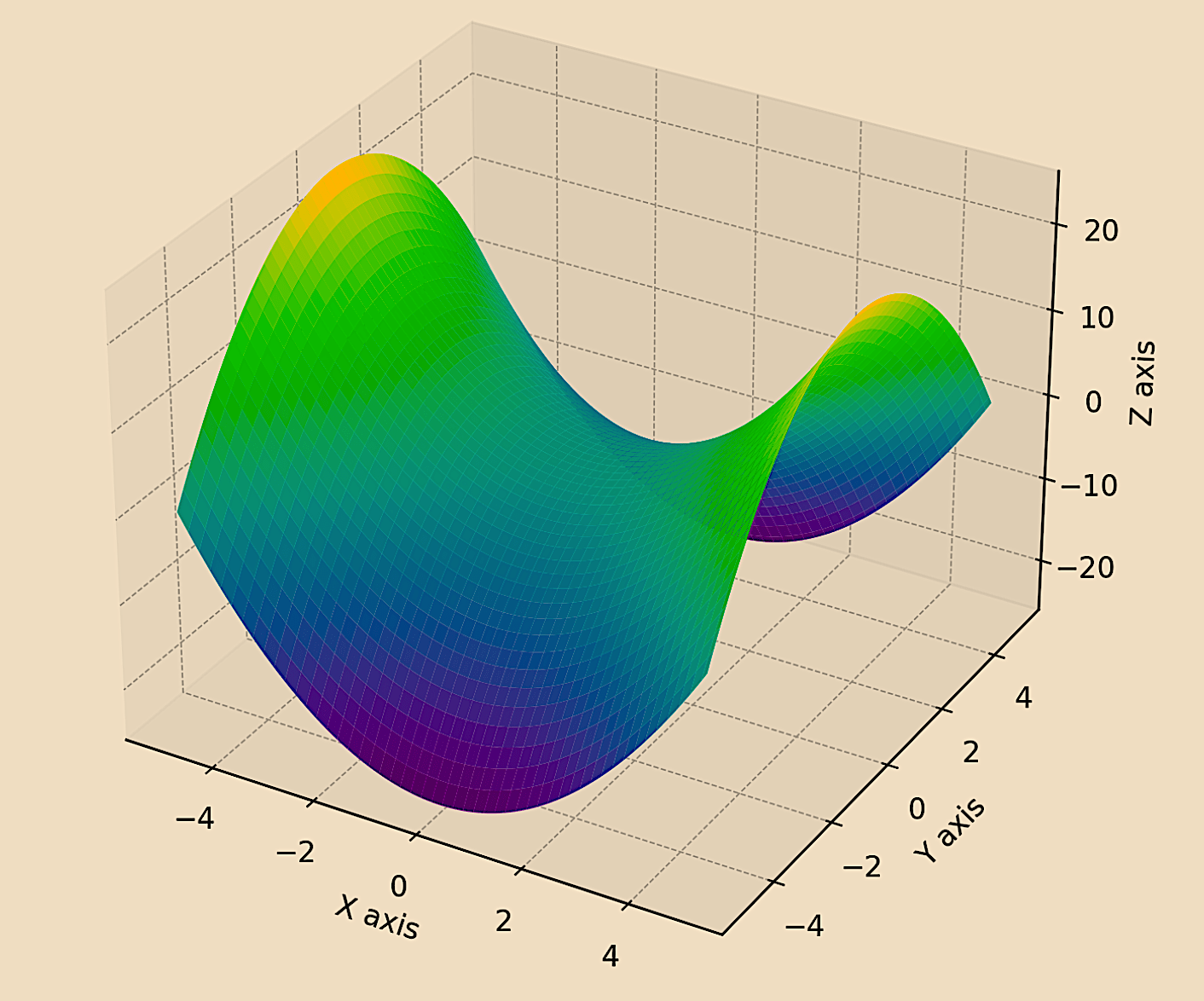
This concept is used in Hamiltonian mechanics.
Phase Space & Poisson Brackets
Phase space provides a unified framework for understanding the state of a mechanical system.
Poisson brackets are used to describe the relationships between dynamical variables in this space.
They offer conceptual tools to understand the dynamic state and evolution of financial systems, and to develop trading algorithms that account for the interplay of various market variables and their momenta.
Quantum Mechanics & Hilbert Spaces
In quantum mechanics, geometric mechanics principles are applied in a probabilistic framework, often using the language of Hilbert spaces and operators.
With their probabilistic frameworks and complex state representations, they’re specifically applied in quantum computing algorithms for finance.
This enables more efficient solutions for optimization problems, portfolio management, and market simulations by leveraging the principles of superposition and entanglement.
Applications in Finance
Risk Management and Portfolio Optimization
Geometric mechanics can be used to understand the dynamics of financial markets and portfolios.
The phase space concept, for instance, can be adapted to visualize and analyze the state of a financial portfolio by considering various factors like asset prices, volatilities, and correlations.
Option Pricing Models
The stochastic differential equations used in option pricing (like the Black-Scholes model) can be analyzed using techniques from geometric mechanics to understand their properties and behavior under different market conditions.
Market Dynamics and Econophysics
Geometric mechanics offers tools to model complex market dynamics, including bubble formation, crashes, and high-frequency trading dynamics.
Quantum Finance
There are emerging applications of quantum mechanics in finance, such as quantum computing for complex financial calculations and modeling.
The principles of geometric mechanics are foundational in understanding these quantum systems.
Algorithmic Trading
Some principles of geometric mechanics can inspire algorithmic strategies.
High-frequency trading where market dynamics can be modeled and predicted with high precision make use of more sophisticated math.
HFT algorithms are typically written in C++ (though a lot of prototyping is done in Python due to the availability of their AI/ML/advanced math libraries).
Limitations
Complexity
The mathematical complexity of geometric mechanics makes it less accessible for typical forms of financial modeling.
Indirect Application
Many of the applications in finance are theoretical or conceptual rather than direct.
Data and Computation
Implementing these concepts practically requires larger amounts of computational resources and highly specialized knowledge.
Geometric Mechanics vs. Differential Geometry vs. Information Geometry in Finance
- Geometric Mechanics deals with dynamic systems and their evolution over time, making it suitable for analyzing dynamic financial markets.
- Differential Geometry is more about the structure and properties of curves and surfaces, useful for understanding the shape and structure of financial data.
- Information Geometry focuses on the probabilistic aspect, treating information (like asset returns) as geometric objects, which is useful in statistical models of finance.
Coding Example – Geometric Mechanics in Finance
In geometric mechanics, a fundamental equation is the Hamiltonian form of the equations of motion.
These equations are used to describe the evolution of a physical system in time and are useful in the context of symplectic geometry, a branch of differential geometry.
The Hamiltonian equations are given by:
- dqi/dt = ∂H/∂pi
- dpi/dt = -∂H/∂qi
Where:
- qi are the generalized coordinates
- pi are the conjugate momenta
- H(qi, pi, t) is the Hamiltonian
- dqi/dt and dpi/dt are the time derivatives of qi and pi
To represent financial data and its momentum stochastically within the Hamiltonian mechanics framework, we’ll interpret the generalized coordinates, as the financial data and the conjugate momenta, as related to the rate of change (momentum) of the data.
The Hamiltonian, can be seen as analogous to the total “energy” of the financial system.
Since real financial systems are subject to “random” external influences, we’ll introduce stochastic elements to both the financial data and its momentum.
This code models the financial data and its momentum using a Hamiltonian-like system with stochastic elements:
import numpy as np

import matplotlib.pyplot as plt

from scipy.integrate import odeint

def stochastic_hamiltonian_system(y, t, sigma_q, sigma_p):
q, p = y
dqdt = p
dpdt = -q + np.random.normal(0, sigma_p) # Stochastic term for momentum
q += np.random.normal(0, sigma_q) # Stochastic term for financial data
return [dqdt, dpdt]

# Initial conditions (q0 = initial data starting point, p0 = initial momentum)
q0 = 1.0
p0 = 0.0

# Standard deviation of the stochastic terms
sigma_q = 0.02 # Randomness in the financial data
sigma_p = 0.02 # Randomness in the momentum

# Time points
t = np.linspace(0, 10, 500)

# Solve the stochastic Hamiltonian system
solution = odeint(stochastic_hamiltonian_system, [q0, p0], t, args=(sigma_q, sigma_p))

# Plotting
plt.figure(figsize=(12, 6))

# Financial data (q)
plt.subplot(1, 2, 1)
plt.plot(t, solution[:, 0])
plt.title('Stochastic Stock Price (q)')
plt.xlabel('Time')
plt.ylabel('Price')

# Momentum (p)
plt.subplot(1, 2, 2)
plt.plot(t, solution[:, 1])
plt.title('Stochastic Momentum (p)')
plt.xlabel('Time')
plt.ylabel('Momentum')

plt.tight_layout()
plt.show()
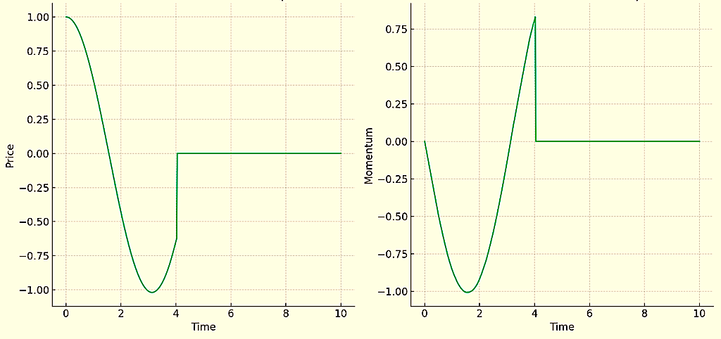
What would this be useful for?
It might be useful for a momentum-based quant trading system where the idea would be to trade momentum after it reaches a certain level or rate of change, expecting it to continue.
It would depend on the trader’s research into the topic/strategy, how they model it algorithmically, and backtesting the algorithm/system thoroughly before deploying it live.