Quantum Finance – Quantum Mechanics Applications in Finance & Trading


Quantum mechanics, a fundamental theory in physics that describes the behavior of matter and energy on the smallest scales, has naturally been confined to science and technology.
However, due to the probabilistic nature of both quantum mechanics and financial markets, quantum principles can also have applications in finance, investing, and trading.
Below we look at the intersection of quantum mechanics and the financial world – quantum finance – exploring how the former can help with problems associated with the latter.
Please note that the parallels we make in this article are more metaphorical. While quantum mechanics and finance are distinct fields, the mathematical principles underlying quantum phenomena can offer unique perspectives and solutions to longstanding challenges in financial markets.
By drawing parallels between these two domains, we can gain deeper insights into market behavior and develop more sophisticated financial models and strategies.
Key Takeaways: Quantum Finance – Quantum Mechanics Applications in Finance & Trading
- Quantum Finance and Classical Physics:
- Quantum mechanics, which describes the behavior of the smallest particles, has potential applications in finance due to its probabilistic nature, similar to the probabilistic nature of financial markets.
- Classical physics deals with the macroscopic world and offers deterministic predictions, while quantum physics, like financial markets, operates on probabilities.
- Foundations and Principles of Quantum Mechanics:
- Quantum mechanics challenges traditional views with three primary principles:
- Wave-particle duality (particles exhibit both wave-like and particle-like behavior)
- Superposition (quantum systems can exist in multiple states at once), and
- Entanglement (particles can be interconnected, affecting each other’s states regardless of distance)
- Quantum Applications in Finance:
- Quantum mechanics offers solutions to modern finance challenges, including portfolio optimization, option pricing, risk assessment, and market predictions.
- Quantum models in finance, such as the Quantum Continuous Model and Quantum Binomial Model, aim to enhance traditional financial models by integrating quantum principles for more accurate results.
Quantum vs. Classical Physics
Quantum physics describes the behavior of the tiniest particles, like atoms and subatomic particles, where phenomena such as superposition and entanglement occur.
Classical physics, on the other hand, deals with the macroscopic world we observe daily, governed by laws like Newton’s laws of motion and Einstein’s theory of gravity (General Relativity).
While classical physics offers deterministic predictions, quantum physics is probabilistic, meaning outcomes are determined by probabilities rather than certainties.
This is much like the financial world, where markets are a function of probabilistic outcomes.
Summary
Within the realm of quantum mechanics, “classical theory” denotes those physical theories that bypass the quantization framework, encompassing classical mechanics and relativity.
Similarly, classical field theories, like general relativity and classical electromagnetism, operate without the principles of quantum mechanics.
Foundations of Quantum Mechanics
Before diving into its applications in finance, it’s important to understand the basics of quantum mechanics.
At its core, quantum mechanics challenges our classical view of the world.
We’ll describe the basic principles below and give a non-finance analogy of each.
Three primary principles define it:
Wave-particle duality
Particles, like electrons, exhibit both wave-like and particle-like behavior.
This duality is central to understanding quantum phenomena.
Analogy
Think of an electron as a dancer who can both waltz (wave-like) and tap dance (particle-like).
Depending on the song (or experiment), the dancer might choose one style over the other, but they’re capable of both.
Superposition
Quantum systems can exist in multiple states simultaneously.
It’s only when we observe these systems that they “collapse” into a single state.
Analogy
Imagine you have a spinning coin.
While it’s in the air, you can’t tell if it’s heads or tails – it’s as if it’s both at the same time.
But once it lands, it clearly shows one side.
That’s like a quantum system being in many states at once until you check it.
Entanglement
Two or more quantum particles can become intertwined in such a way that the state of one particle directly affects the state of the other, regardless of the distance between them.
Analogy
Picture two magic dice.
No matter how far apart you take them, when you roll one and it shows a 6, the other will instantly show a 1, even if it’s miles away.
They’re mysteriously linked, so one always knows what the other is doing.
Interdisciplinary Example: Wave Function in Quantum Mechanics vs. Probability Distributions of Asset Returns in Finance
Wave functions in quantum mechanics and probabilistic distributions in finance might seem like concepts from entirely different realms.
But they share a foundational similarity: both describe uncertainties and probabilities.
Wave Functions in Quantum Mechanics
- A wave function, often denoted by the Greek letter ψ (psi), represents the state of a quantum system.
- The square of its magnitude, |ψ|^2, gives the probability density of finding a particle in a particular state or position.
- When you measure a quantum system, the wave function “collapses” to a specific value, but until that measurement, the system exists in a superposition of all possible states.
- Thus, the wave function provides a probabilistic description of the system.
Probabilistic Distribution in Finance
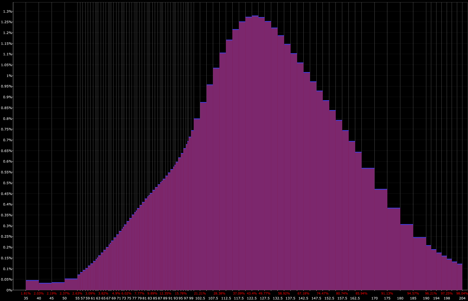
- In finance, especially when dealing with asset price returns, we often use probabilistic distributions to describe where an asset price (or another variable) could be by a certain time (see below).
- For instance, the future return on an asset is uncertain, and we might use a certain type of distribution (normally with fatter tails than a normal distribution) to describe the range of possible returns and their associated probabilities.
- Just as the wave function gives the likelihood of a particle being in a particular state, the probabilistic distribution in finance gives the likelihood of an asset achieving a particular return.
The Analogy
Imagine you’re trying to predict the stock price for a company at a certain point in the future.
You can’t know for sure what the price will be, but based on historical data and other factors, you can assign probabilities to different potential prices.
This is similar to a quantum particle whose position isn’t determined until measured.
Before measurement, the particle’s position is described by a wave function that assigns probabilities to various positions.
In both cases, the systems (the quantum particle and the stock price) are governed by inherent uncertainties.
Quantum mechanics uses wave functions to describe these uncertainties, while finance uses probabilistic distributions.
The key similarity is that both provide a framework to understand and quantify the unknown.
A Simple Explanation of Quantum Wavefunctions
Math in Quantum Mechanics and Applications in Financial Markets
Quantum mechanics is rooted deeply in mathematics.
The mathematical formulations that describe quantum phenomena are intricate, but they can be analogously applied to financial markets to provide insights and solutions to complex financial problems.
Let’s look into some of the fundamental mathematical concepts of quantum mechanics and explore their potential applications in finance.
Schrödinger Equation
The Schrödinger equation, at its core, describes the evolution of a system over time based on certain initial conditions and constraints.
While it was developed to describe quantum systems, the mathematical structure can be at least metaphorically applied to financial markets.
Here’s how:
Particle in a Box & a Security in a Financial Market
In quantum mechanics, a particle in a box is confined to a certain space and its energy levels are quantized.
Similarly, a financial asset’s price might be confined within certain levels due to market factors, regulations, or other constraints.
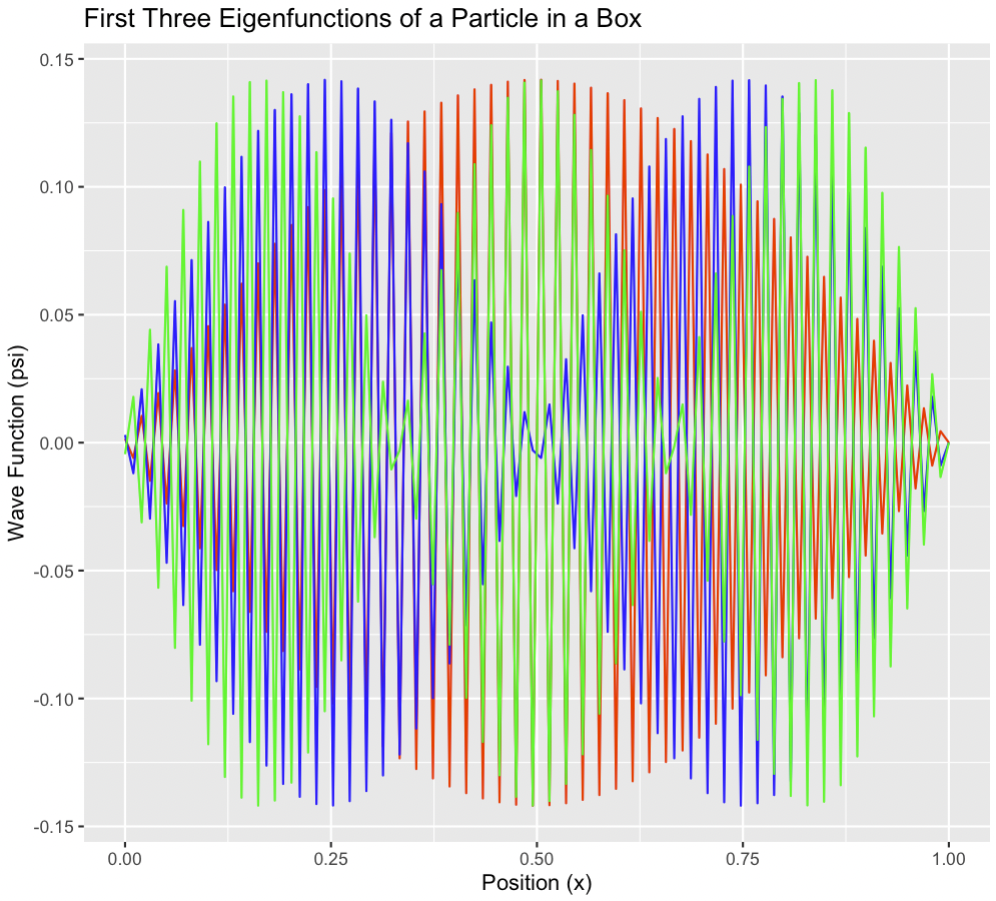
The eigenfunctions (wave functions) of the particle represent different states the particle can be in.
In finance, these could metaphorically represent different states or scenarios for an asset, such as uptrends, downtrends, or sideways markets.
In terms of a diagram, this might look like the following:
The R Code for producing this:
# Constants
hbar <- 1  # Reduced Planck constant (set to 1 for simplicity)
m <- 1     # Particle mass (set to 1 for simplicity)
L <- 1     # Length of the box

# Discretize the spatial domain
N <- 100
dx <- L / (N-1)
x <- seq(0, L, by=dx)

# Construct the Hamiltonian matrix
H <- matrix(0, N, N)
for (i in 2:(N-1)) {
  H[i, i-1] <- H[i, i+1] <- 1
  H[i, i] <- -2
}

H <- -hbar^2 / (2 * m * dx^2) * H

# Solve for eigenvalues and eigenvectors
eigenvalues <- eigen(H, symmetric=TRUE)$values
eigenvectors <- eigen(H, symmetric=TRUE)$vectors

# Plot the first few eigenfunctions
library(ggplot2)
data <- data.frame(x=x, psi1=eigenvectors[,1], psi2=eigenvectors[,2], psi3=eigenvectors[,3])
ggplot(data, aes(x=x)) +
  geom_line(aes(y=psi1), color="red") +
  geom_line(aes(y=psi2), color="blue") +
  geom_line(aes(y=psi3), color="green") +
  ggtitle("First Three Eigenfunctions of a Particle in a Box") +
  ylab("Wave Function (psi)") +
  xlab("Position (x)")
(Explanation: The Schrödinger equation is a partial differential equation, and solving it numerically requires discretizing the spatial domain and time-stepping. We used a simple example of solving the time-independent one-dimensional Schrödinger equation using finite difference methods in R. This code sets up and solves the time-independent Schrödinger equation for a particle in a box of length using finite difference methods. The resulting plot above shows the first three eigenfunctions (wave functions) of the particle, which correspond to the three lowest energy states. The eigenvalues would give the energy levels of these states.)
Probability Distributions
The square of the wave function in quantum mechanics gives a probability distribution of finding a particle in a certain position.
Similarly, in finance, we often deal with probability distributions to model uncertainties (i.e., lots of possibilities with different probabilities associated with them), such as the likelihood of different returns on an asset.
The peaks in the eigenfunctions could represent times of high probability or high activity for an asset, while troughs could represent low activity.
Using what we have above, we can square these wave functions to derive the probability densities:
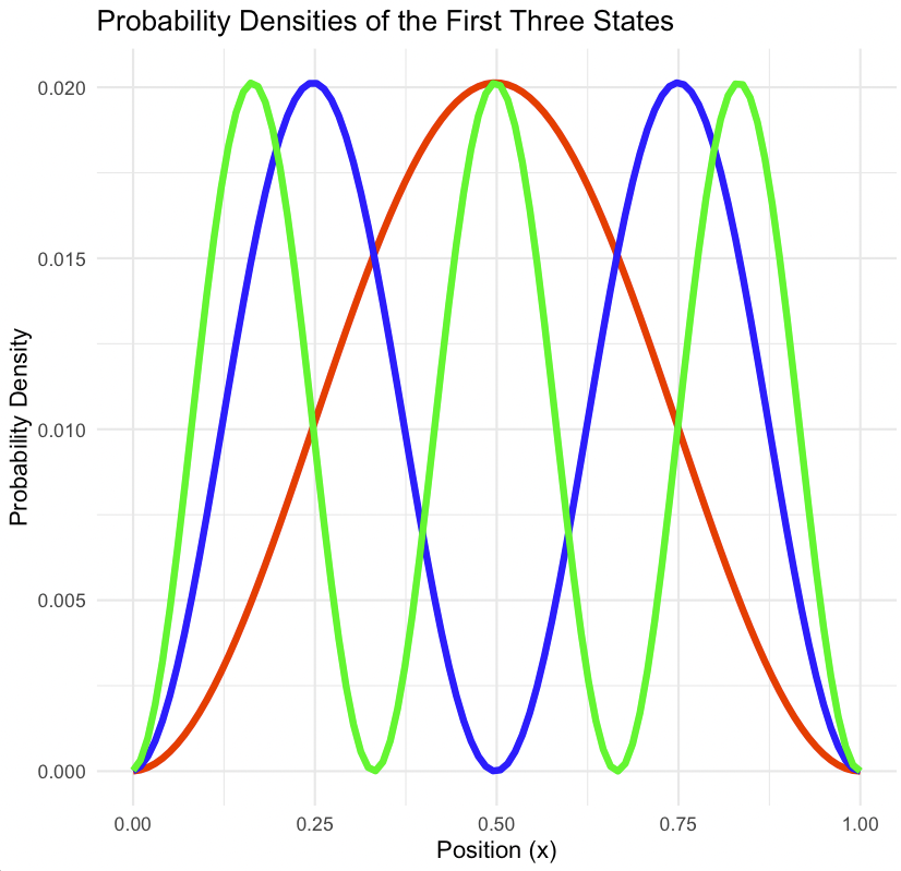
Analogously, in financial markets, the probability densities would be akin to the odds of finding the asset at that particular price at a certain point in the future.
The code for doing this in R:
# Constants
hbar <- 1  # Reduced Planck constant (set to 1 for simplicity)
m <- 1     # Particle mass (set to 1 for simplicity)
L <- 1     # Length of the box

# Discretize the spatial domain
N <- 100
dx <- L / (N-1)
x <- seq(0, L, by=dx)

# Construct the Hamiltonian matrix
H <- matrix(0, N, N)
for (i in 2:(N-1)) {
  H[i, i-1] <- H[i, i+1] <- 1
  H[i, i] <- -2
}
H <- -hbar^2 / (2 * m * dx^2) * H

# Solve for eigenvalues and eigenvectors
eigenvalues <- eigen(H, symmetric=TRUE)$values
eigenvectors <- eigen(H, symmetric=TRUE)$vectors

# Compute the squared wave functions
prob_density1 <- eigenvectors[,1]^2
prob_density2 <- eigenvectors[,2]^2
prob_density3 <- eigenvectors[,3]^2

# Plot the squared wave functions
library(ggplot2)
data <- data.frame(x=x, prob_density1=prob_density1, prob_density2=prob_density2, prob_density3=prob_density3)
ggplot(data, aes(x=x)) +
  geom_line(aes(y=prob_density1), color="red", lwd=1.5) +
  geom_line(aes(y=prob_density2), color="blue", lwd=1.5) +
  geom_line(aes(y=prob_density3), color="green", lwd=1.5) +
  ggtitle("Probability Densities of the First Three States") +
  ylab("Probability Density") +
  xlab("Position (x)") +
  theme_minimal()
(Explanation: The square of the wave function, , gives the probability density of finding a particle at position . In the context of the particle in a box problem we discussed earlier, we can plot for the first few eigenfunctions to visualize the probability distribution. This code computes the squared wave functions (probability densities) for the first three eigenfunctions of a particle in a box and plots them. The peaks in the plots represent positions where the particle is most likely to be found, while the troughs represent positions where the particle is least likely to be found.)
Superposition & Portfolio Makeup
Quantum superposition, where a system can exist in multiple states simultaneously, can be likened to a diverse financial portfolio.
Each asset in the portfolio can be thought of as being in a superposition of different states of returns.
Just as measuring a quantum system collapses the superposition, making a financial decision based on certain information can “collapse” the potential outcomes into a realized return.
Potential Wells & Market Barriers
In quantum mechanics, potential wells can confine or repel a particle.
Similarly, in finance, there are barriers such as regulations, market sentiment, or major news events that can confine or influence asset prices.
Time Evolution & Forecasting
The time-dependent Schrödinger equation describes how a system evolves over time.
In finance, forecasting models aim to predict how assets or markets will evolve over time based on current and past data.
Quantum Tunneling & Market Breakouts
In quantum mechanics, there’s a phenomenon called quantum tunneling where particles can pass through barriers that classical physics says they shouldn’t.
Drawing a parallel in finance, there are times when assets or markets break through price barriers or resistances in unexpected ways (even relative to their probabilistic distributions), often due to unforeseen news or events.
Heisenberg Uncertainty Principle
This principle states that certain pairs of physical properties (like position and momentum) cannot both be precisely measured simultaneously.
The more precisely one property is known, the less precisely the other can be known.
Application in Finance
In financial markets, there’s always a trade-off between various things.
The Heisenberg Uncertainty Principle can be analogously applied to model a financial trade-off.
For example:
- the more certain an investor is about the expected return of an asset, the less risk they are generally taking on and the more in future return they may be forgoing
Quantum Entanglement
When two quantum particles become entangled, the state of one particle instantly affects the state of the other, no matter the distance between them.
Application in Finance
In global financial markets, assets and indices can be “entangled” in the sense that a change in one market or asset class can instantaneously affect another.
This can be used to model and understand global financial interdependencies, covariances, and correlations, aiding in portfolio diversification and risk management.
Quantum Superposition
Quantum systems can exist in a combination of multiple states simultaneously until observed.
Application in Finance
Financial assets, especially in complex derivatives markets, can be thought of as existing in multiple potential states (e.g., various potential payoffs) until “observed” or realized at expiration.
This concept can be used to model and price complex financial instruments.
Examples of Quantum Principles in Finance
Let’s look at some additional examples.
Portfolio Optimization using Superposition
Just as a quantum system can exist in multiple states, a portfolio can be thought of as a superposition of various asset combinations.
Quantum algorithms can then sift through these combinations to find the optimal mix that maximizes returns for a given risk level.
And do this in a dynamic way – i.e., there may be no static allocation that does this.
However, in the real-world transaction costs matter.
Entangled Asset Correlations
Consider two major stock indices, such as the S&P 500 and the Nikkei 225.
A significant geopolitical event affecting the US market might instantaneously impact the Japanese market, even if the actual economic implications for Japan are not immediately clear.
This instantaneous correlation can be modeled using principles similar to quantum entanglement.
Summary
Quantum mechanics may not directly apply to finance, but the mathematical structures and concepts can inspire new ways of thinking about financial markets and modeling them in a more robust way.
Path Integrals in Quantum Mechanics and Their Application to Finance
Path integrals, also known as Feynman integrals, were introduced by Richard Feynman as an alternative formulation of quantum mechanics.
Instead of describing quantum systems using wave functions or matrices, the path integral approach considers all possible paths a particle can take between two points in spacetime.
Concept
The basic idea is to sum (or integrate) over all possible trajectories or paths that a particle can take from point A to point B.
Each path is assigned a probability amplitude, and the sum of these amplitudes gives the total probability amplitude for the particle to move from A to B.
Mathematical Representation
The path integral is represented as an integral over all possible paths, where each path is weighted by a phase factor given by the exponential of the action (a quantity derived from the Lagrangian of the system) for that path.
Significance
Path integrals provide a more intuitive understanding of quantum mechanics, especially in quantum field theory and particle physics.
They are particularly useful in systems where traditional methods are cumbersome or intractable.
Application to Finance and Financial Markets
The concept of considering all possible paths or trajectories can be analogously applied to financial markets, especially in the context of derivative pricing and risk management.
Market Outcomes
Market outcomes in the future are modeled via probability distributions.
Integration can be applied to probability spaces to find the probability of what an asset or portfolio’s returns will be by a certain point in the future.
Option Pricing
When pricing options, especially exotic options, one needs to consider all possible paths the underlying asset can take until the option’s expiration.
The path integral approach can be used to sum over all these paths, each weighted by a certain probability, to determine the option’s fair value.
This is similar to the Monte Carlo simulation method of options pricing, where multiple asset price paths are simulated to price complex derivatives.
Risk Management
In risk management, especially Value at Risk (VaR) calculations, firms need to consider all possible market scenarios or paths to assess potential losses.
The path integral framework can provide a mathematical foundation for considering all these scenarios and their associated probabilities.
Market Dynamics and Evolution
Financial markets evolve over time, influenced by a myriad of factors.
The path integral approach can be used to model the evolution of market variables by considering all possible trajectories they can take, given current information and market conditions.
Portfolio Optimization
Just as path integrals consider all possible trajectories of a particle, they can be used to consider all possible portfolio combinations when optimizing a portfolio.
Each portfolio combination or path can be assigned a probability based on expected returns and risks, and the optimal portfolio can be determined by summing over these paths.
Examples
Some examples:
Interest Rate Modeling
Interest rates have multiple potential future paths based on various economic scenarios.
The path integral approach can be used to model the evolution of interest rates by considering all these potential paths, aiding in the pricing of interest rate derivatives.
Stock Price Evolution
For a stock option that depends on the entire price path of the underlying stock (e.g., Asian options), the path integral method can be used to consider all possible stock price trajectories until expiration, helping in accurate option pricing.
Summary
While path integrals originate from quantum mechanics, their conceptual framework of considering all possible paths or trajectories finds analogous applications in finance.
By adopting such quantum-inspired methods, traders, investors, financial analysts, and researchers can develop more robust models and strategies for navigating financial markets and various financial phenomena.
Quantum Computing Basics
Quantum computing, inspired by quantum mechanics, promises computational power far surpassing that of classical computers.
Here’s a brief overview:
Quantum bits (qubits) vs. classical bits
While classical bits can be either 0 or 1, qubits can exist in a superposition of both states, allowing for more complex computations.
Quantum gates and circuits
Just as classical computers use logic gates to perform operations on bits, quantum computers use quantum gates to manipulate qubits.
Quantum algorithms
These are specific procedures designed for quantum computers.
Notable examples include Grover’s algorithm, which can search databases faster than classical methods, and Shor’s algorithm, which can factor large numbers efficiently.
Challenges in Modern Finance
Modern finance faces several challenges, leading to interest in quantum computing:
Complexity of financial markets
Financial markets have become interconnected over time, and new products and participants make them more complex.
This means that markets become more technologically- and resource-intensive to “figure out.”
Limitations of classical computational models
Traditional models often struggle to process vast amounts of data quickly or simulate complex financial systems accurately.
Need for faster and more efficient algorithms
More and more financial data is available as time goes on.
Naturally, there’s a growing demand for algorithms that can keep up.
Quantum Algorithms in Finance
Quantum mechanics offers solutions to some of the challenges faced by modern finance.
Here are some areas where quantum algorithms can make a difference:
Portfolio optimization
Quantum algorithms can sift through vast datasets to find the optimal mix of assets for a particular purpose (e.g., goals, time horizon, risk tolerance), maximizing returns while minimizing risks.
Option pricing
Quantum methods can calculate the value of financial options more quickly and accurately than classical methods.
Risk assessment and management
Quantum computing can simulate complex financial systems, helping institutions understand potential risks and devise strategies to mitigate them.
Forecasting and prediction
With their computational power, quantum computers may be able to analyze market trends and make predictions with higher accuracy.
Quantum Models in Finance
Let’s look into some quantum models in trading and finance:
Quantum Continuous Model
This model is an adaptation of the classical continuous-time finance models to the quantum framework.
In classical finance, continuous models like the Black-Scholes model are used to price options by considering the continuous change in asset prices.
In the quantum continuous model, quantum mechanics principles are applied to these continuous changes, allowing for more complex and potentially more accurate modeling of financial systems.
Quantum Binomial Model
The binomial model in classical finance is a discrete-time model used for option pricing, where the underlying asset can take one of two possible values in the next time step.
The quantum binomial model introduces quantum principles into this framework.
Instead of having definite asset values, the quantum version considers superpositions of possible asset values, leading to a richer set of possible outcomes and potentially more accurate pricing.
Multi-step Quantum Binomial Model
Building on the quantum binomial model, the multi-step version considers multiple time steps into the future.
This allows for a more detailed and nuanced representation of how an asset’s price might evolve over time.
By considering multiple steps, this model can capture a broader range of potential market dynamics and offer more detailed insights into option pricing and risk assessment.
Quantum Algorithm for the Pricing of Derivatives
Derivatives are financial instruments whose value is derived from an underlying asset.
Pricing them accurately is important for financial markets.
Classical algorithms can be computationally intensive, especially for complex or exotic derivatives.
Quantum algorithms leverage the principles of quantum mechanics to speed up the computation process.
Using concepts like quantum superposition and entanglement, these algorithms can evaluate multiple pricing scenarios simultaneously, leading to faster and potentially more accurate pricing of derivatives.
Quantum options pricing will give different results than options pricing using classical models (e.g., Cox-Ross-Rubinstein or Hull-White and Cox-Ingersoll-Ross in the context of rates derivatives).
This is because in a quantum application, the underlying asset is treated like, e.g., a quantum boson particle (Bose-Einstein assumption) rather than a classical particle.
Summary
In essence, these quantum applications aim to enhance traditional financial models by incorporating the unique principles of quantum mechanics.
By doing so, they offer the potential for more accurate modeling, pricing, and risk assessment.
Quantum Machine Learning in Trading
Machine learning, with its ability to analyze and make predictions from vast datasets, has already made significant inroads in trading.
Quantum mechanics takes this a step further with quantum-enhanced machine learning models:
Quantum-enhanced machine learning models
These models leverage the principles of superposition and entanglement to process information in ways classical models can’t.
This means they can potentially recognize patterns and make predictions faster and more accurately.
Quantum neural networks
Just as classical neural networks are the backbone of many machine learning applications, quantum neural networks (QNNs) are their quantum counterparts.
QNNs can process a vast amount of information simultaneously, making them particularly suited for real-time trading applications.
Trading strategy optimization using quantum algorithms
Traders are always on the lookout for the best strategies to maximize their returns at reasonable risk levels.
Quantum algorithms can analyze multiple strategies at once.
This helps traders identify the most promising ones in a fraction of the time it would take classical algorithms.
Practical Implementations
The theoretical benefits of quantum mechanics in finance are clear, but how about practical applications?
Here’s are some ideas into the real-world implementations:
Quantum hardware
The foundation of any quantum application is the hardware.
Technologies like superconducting qubits and trapped ions are leading the way.
Companies and research institutions are working on making them more accessible and scalable.
Quantum software platforms and libraries
As the hardware evolves, so does the software.
Platforms and libraries tailored for quantum applications in finance are emerging.
These can make it easier for financial institutions to integrate quantum solutions into their operations.
Case studies
Several financial institutions have already begun experimenting with quantum technologies.
For instance, some banks are using quantum algorithms to optimize their asset portfolios, while hedge funds are exploring quantum-enhanced trading strategies.
Challenges and Limitations
While quantum mechanics holds immense promise for finance and trading, it’s not without its challenges:
Scalability issues
Building large-scale quantum computers that can handle complex financial applications is still a challenge.
Current quantum computers are often termed “noisy intermediate-scale quantum” (NISQ) devices, indicating their limitations.
Quantum vs. classical
It’s important to determine when it’s beneficial to use quantum algorithms over classical ones.
Not all financial problems will benefit from a quantum approach.
Future Prospects
Here are some ideas into what the future might hold:
Evolution of quantum hardware and software
As research goes on, we can expect quantum computers to become more powerful, reliable, and accessible.
This evolution will be complemented by the development of quantum software platforms tailored for financial applications.
Potential breakthroughs in quantum algorithms for finance
As the field matures, researchers will likely discover new quantum algorithms that can address financial challenges more efficiently than before.
Integration of quantum technologies with AI and other emerging tech
The future of finance won’t just be shaped by quantum mechanics alone.
The integration of quantum technologies with artificial intelligence, blockchain, and other emerging technologies can lead to hybrid solutions that use the strengths of each domain.
What is Quantum Information Theory in Physics and Its Applications to Finance and Trading?
Information theory, originally developed by Claude Shannon for telecommunications, deals with the quantification of information.
In physics, it’s used to understand the flow and storage of information in physical systems, especially in the realms of thermodynamics and quantum mechanics.
Thermodynamics
The concept of entropy in thermodynamics describes the amount of disorder in a system
It is closely related to Shannon’s entropy in information theory, which measures the amount of uncertainty or surprise associated with random variables.
Quantum Mechanics
Quantum information theory explores how quantum systems store and process information.
Concepts like quantum entanglement can be understood in terms of information being shared between quantum states.
Application to Finance and Trading
- Efficient Data Transmission: Financial markets pricing is based on the processing of vast amounts of data. Information theory can help in the efficient encoding, transmission, and decoding of this data. This can ensure that trading algorithms receive timely and accurate market data.
- Risk and Uncertainty: Shannon’s entropy could be used analogously to quantify the uncertainty in financial models. A higher entropy might indicate a more unpredictable security, asset, or market, guiding traders and investors in risk assessment.
- Optimal Portfolio Construction: By quantifying the amount of information or uncertainty in various assets, traders can construct portfolios that maximize returns for a given level of risk.
- Algorithmic Trading: Trading algorithms can be optimized using principles from information theory to ensure they’re making decisions based on the most relevant and actionable information.
- Market Dynamics: Information theory can help understand how information flows in financial markets, how quickly it’s incorporated into prices, and how anomalies like bubbles or crashes might arise from information asymmetries.
Information theory provides tools to quantify and manage uncertainty, making it valuable in the probabilistic nature of finance, investing, and trading.
FAQs – Quantum Finance & Quantum Applications in Finance and Trading
What is quantum finance?
Quantum finance is the interdisciplinary field that integrates principles of quantum mechanics into financial modeling and decision-making.
It seeks to improve the accuracy and efficiency of financial models by leveraging the unique properties of quantum systems, such as superposition and entanglement.
What is quantum volatility in the context of financial markets?
Quantum volatility refers to a modeling approach that uses quantum mechanics to describe the uncertainties and fluctuations in financial markets that leads to asset price volatility.
Traditional volatility models might not capture all the complexities of market behavior.
Quantum volatility models aim to provide a more nuanced representation by incorporating quantum principles, potentially offering a better understanding of price fluctuations and risks.
How are quantum algorithms different from classical algorithms in finance?
Quantum algorithms leverage the principles of quantum mechanics, such as superposition (where a quantum system can exist in multiple states simultaneously) and entanglement (where particles become interconnected).
This allows quantum algorithms to process vast amounts of information simultaneously and solve certain problems much faster than classical algorithms.
In finance, this can lead to quicker and more accurate pricing, optimization, and risk assessment.
How can quantum mechanics be applied to the pricing of options and derivatives?
Quantum mechanics can enhance the models used for pricing options and derivatives.
For instance, the quantum binomial model is a quantum version of the classical binomial model for option pricing.
By considering superpositions of asset prices, quantum models can capture a broader range of potential market dynamics, leading to potentially more accurate pricing.
Additionally, quantum algorithms can speed up the computational process of pricing complex derivatives.
What are superpositions of asset prices?
Superpositions of asset prices refer to the quantum concept where an asset doesn’t have a definite price but exists in multiple possible price states simultaneously.
Just as a quantum particle can be in a superposition of different states until observed, an asset’s price, in a quantum model, can be in a blend of several potential values.
Only when “measured” or observed does it collapse to a specific price.
How are path integrals used in quantum mechanics and how can they be applied to finance and financial markets?
Path integrals in quantum mechanics represent the summation of all possible histories a system can take between two states, providing a probabilistic framework for quantum transitions.
As we explained in other sections of this article, in finance, the concept is analogous to evaluating all possible paths an asset’s price can take over time. (We have a distribution.)
By using path integrals, financial analysts can model the evolution of asset prices in complex markets, taking into account various stochastic processes and uncertainties.
This approach aids in option pricing, risk assessment, and other financial analyses by offering a comprehensive view of potential market behaviors.
How can the Schrödinger Equation be applied to financial contexts?
The Schrödinger equation describes how the quantum state of a physical system changes over time.
It is central to quantum mechanics and provides a probabilistic prediction of a system’s future behavior.
Schrödinger equation application in Finance
In finance, asset prices are also “systems” that change over time influenced by various factors.
The probabilistic nature of the Schrödinger equation can be used to model asset price movements, where the “quantum state” of an asset represents its price.
For example, the future price of a security or asset can be thought of as a superposition of various potential prices, much like a quantum state before measurement.
How can a wave function, ψ (psi), be applied to financial markets?
The wave function represents the state of a quantum system.
The square of its magnitude, |ψ|^2, gives the probability density of finding a particle in a particular state or position.
Wave function application in Finance
The wave function’s probabilistic interpretation can be applied to financial instruments.
For instance, the likelihood of an asset achieving a particular return can be modeled using a “financial wave function.”
This can be particularly useful in options pricing, where the payoff depends on the underlying asset’s price at expiration.
It can also model specific asset returns or entire portfolio returns.
How can quantum mechanics principles be applied to computational finance?
In computational finance, where vast amounts of data need to be processed and complex simulations are run, quantum mechanics offers several advantages:
- Speed: Quantum algorithms can solve certain problems faster than their classical counterparts.
- Complex Modeling: Quantum systems can model complex financial systems in superposition, capturing a wider range of potential scenarios.
- Optimization: Quantum algorithms can be used for tasks like portfolio optimization, finding the best mix of assets more efficiently.
- Machine Learning: Quantum-enhanced machine learning models can analyze market data more effectively, leading to better predictions and strategies.
How can wave-particle duality, superposition, and entanglement be applied to financial markets (e.g., asset returns, risk, portfolio construction and optimization)?
The application of quantum concepts like wave-particle duality, superposition, and entanglement to financial markets is still exploratory.
Here’s a simplified breakdown of how these principles might be applied:
Wave-Particle Duality and Financial Markets
- Asset Returns: Just as particles exhibit both wave-like and particle-like behavior, asset returns can be viewed in terms of both continuous (wave-like) price movements and discrete (particle-like) events or shocks. Moreover, you never know what the future price of an asset is until it’s measured at a particular point in time, which yields a distribution much like wave functions as described by the Schrödinger equation.
- Risk: Wave-particle duality can help in modeling market uncertainties by considering both continuous risk (market trends) and discrete risk (sudden market events).
Superposition in Finance
- Asset Returns: Instead of an asset having a deterministic future price, it can be considered to exist in a superposition of multiple potential future prices. This can provide a richer model for understanding unknowns in prices.
- Portfolio Construction and Optimization: Portfolios can be constructed considering a “superposition” of multiple asset combinations. Quantum algorithms can then be used to quickly find the optimal combination that maximizes returns for a given risk level.
Entanglement and Financial Markets
- Asset Correlations: In traditional finance, assets are generally correlated to some degree, meaning the price of one can influence another. Quantum entanglement can offer a deeper level of correlation, where the state of one asset instantly affects another, regardless of distance or other intervening factors. This can provide a more nuanced understanding of asset relationships.
- Portfolio Optimization: Entangled states can be used to represent complex financial instruments or strategies. Understanding these entanglements can lead to better portfolio diversification and risk management.