Variational Bayesian Methods in Finance, Markets & Trading

Variational Bayesian methods, within the context of probability theory in finance and markets, offer a framework for dealing with uncertainty and making predictions.

These methods belong to the family of Bayesian inference techniques, which update the probabilities of hypotheses as more evidence becomes available.

Variational Bayesian methods specifically use optimization techniques to approximate complex posterior distributions and provide a computationally efficient alternative to traditional sampling methods like Markov Chain Monte Carlo (MCMC).

Key Takeaways – Variational Bayesian Methods in Finance, Markets & Trading

• Efficient Approximation
  • Variational Bayesian methods provide an efficient way to approximate posterior distributions in financial models.
  • Enables faster and scalable inference compared to traditional sampling methods.
• Uncertainty Quantification
  • These methods allow for the quantification of uncertainty in estimates and predictions.
• Model Complexity Management
  • Variational Bayesian approaches facilitate the use of more complex models by simplifying the inference process.
  • This allows traders and analysts to capture market dynamics and relationships better.

Here’s how these methods are applied in finance and markets:

Portfolio Optimization

In portfolio optimization, traders/investors generally aim to allocate their assets in a way that maximizes returns for a given level of risk.

Variational Bayesian methods can be used to estimate the posterior distributions of asset returns.

This takes into account not only the historical returns but also the uncertainty in those estimates (i.e., represented as a probability distribution).

This allows for better optimization under uncertainty, which helps traders/investors to make more informed allocation decisions.

Risk Management

Risk management involves assessing and controlling (or eliminating) financial risks.

Variational Bayesian methods can model the uncertainty of relevant risk factors, such as market volatility, interest rates, or credit risk.

By approximating the posterior distributions of these risk factors, financial institutions can better understand the range of possible outcomes and the probabilities of extreme events.

Algorithmic Trading

Algorithmic trading strategies often rely on predictive models to make trading decisions.

Variational Bayesian methods can be used to develop predictive models that incorporate uncertainty about market conditions, asset prices, or the impact of economic indicators.

This probabilistic approach allows trading algorithms to not only make predictions about future market movements but also quantify the confidence in those predictions.

Many, many things are possible. It’s the probabilities that matter.

Credit Scoring

Credit scoring involves predicting the probability of default on loans.

Variational Bayesian methods can be applied to model the uncertainty in borrowers’ creditworthiness.

This incorporates various financial indicators and personal information.

By estimating the posterior distributions of default probabilities, lenders can make more nuanced lending decisions that account for the inherent uncertainty in creditworthiness.

Asset Pricing

Asset pricing models seek to determine the fair value of financial instruments.

Variational Bayesian methods can enhance these models by incorporating uncertainty into the pricing process, such as the uncertainty in model parameters or in future cash flows.

This allows for a probabilistic assessment of asset prices.

This provides a range of possible values and their associated probabilities rather than a single point estimate.

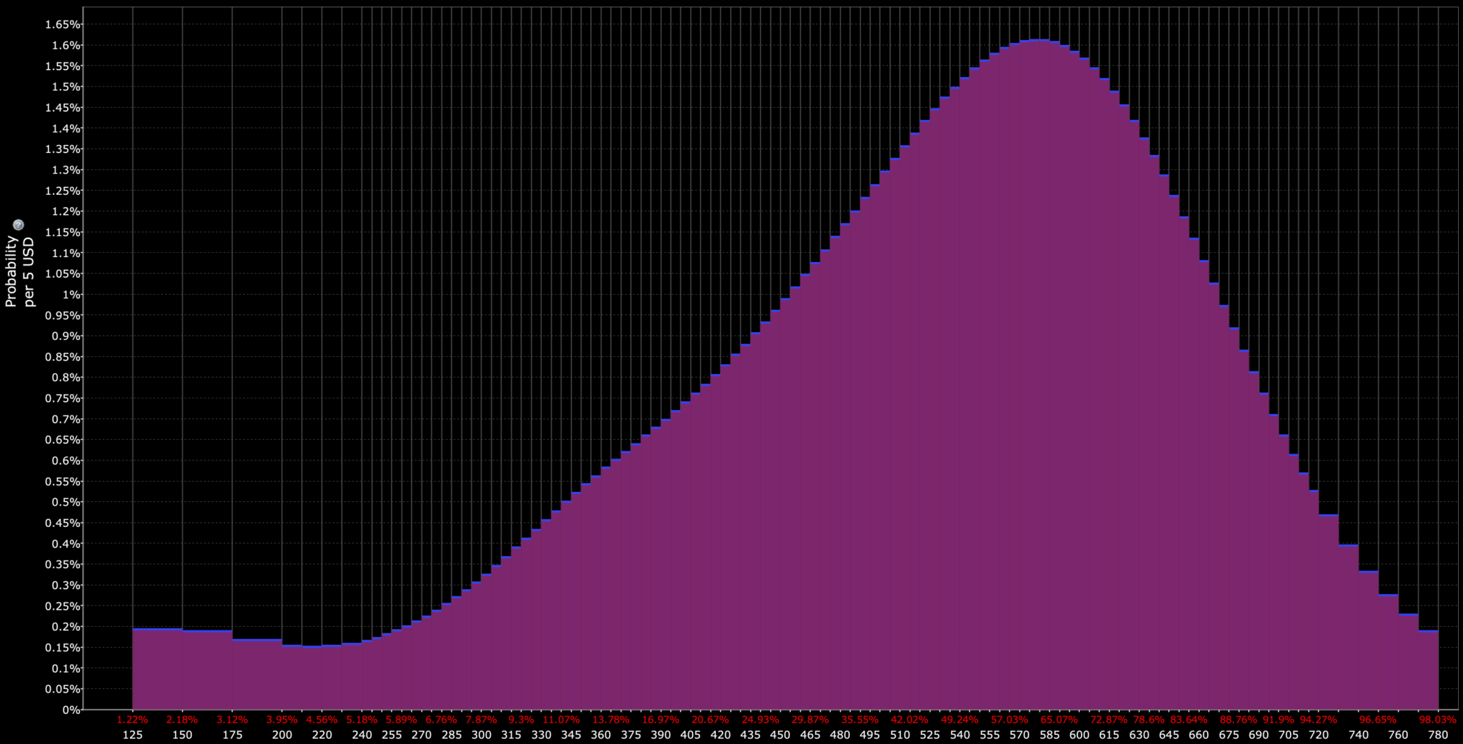
When viewing things in terms of probability distributions, you know that a wide range of outcomes is possible.

For example, in the probability distribution below, even the most probable prices (at or around the peak) have less than a 2% chance of being the result.

Advantages and Challenges

Advantages

• Computational Efficiency – Variational Bayesian methods are generally more computationally efficient than sampling-based methods (especially in large-scale applications or when real-time analysis is required).
• Handling of Uncertainty – These methods provide a systematic way to incorporate and quantify uncertainty. Sheds insights into the probability distributions of model parameters or predictions.

Challenges

• Approximation Bias – Variational methods involve approximating the true posterior distributions, which can introduce bias if the chosen family of distributions isn’t flexible enough to capture the true complexity.
• Model Complexity – Developing and implementing variational Bayesian models can be complex. It requires careful consideration of the model structure and the optimization process.

Variational Bayesian Methods vs. Traditional Bayesian Methods

The term “variational” in the context of variational Bayesian methods refers to a computational approach used to approximate probability distributions in Bayesian statistics.

Let’s break down the concept and how it differs from traditional Bayesian methods:

Traditional Bayesian Methods

Bayesian methods revolve around Bayes’ theorem, which updates the probability estimate for a hypothesis as more evidence becomes available.

An example would be updating your impressions of how a stock would be valued after quarterly earnings is released.

Bayesian methods calculate the posterior distribution, which combines prior beliefs about a parameter with the likelihood of observing the data given those parameters.

For complex models, this posterior distribution can be very difficult to compute exactly because it involves high-dimensional integrals over the parameter space.

Traditional Bayesian methods, like Markov Chain Monte Carlo (MCMC), tackle this challenge by using sampling techniques.

They generate samples from the posterior distribution and use these samples to estimate properties of the distribution (such as its mean or variance).

MCMC methods can be very accurate, but they’re often computationally intensive and slow – especially true for complex models or large datasets.

Variational Bayesian Methods

“Variational” refers to the use of optimization techniques to find the best approximation of the posterior distribution from within a specific family of simpler distributions.

Instead of sampling from the posterior directly, variational Bayesian methods approximate it with a distribution that is easier to handle computationally.

The “best” approximation is found by minimizing the difference between the true posterior and the approximating distribution, typically measured by a divergence metric like the Kullback-Leibler (KL) divergence.

Key Differences

• Computational Efficiency – Variational methods are generally faster than MCMC and other sampling methods because they turn the problem of Bayesian inference into an optimization problem, which can be solved more efficiently.
• Approximation vs. Sampling – Variational Bayesian methods approximate the posterior distribution directly, while traditional Bayesian methods rely on sampling to estimate the properties of the posterior.
• Trade-off – The speed and efficiency of variational methods come at the cost of accuracy. The approximation may not capture all the nuances of the true posterior distribution. This may introduce some bias into the inference.

Variational Bayesian Methods for Portfolio Optimization

You can use variational Bayesian methods to analyze historical asset price data for predicting future distributions and optimizing portfolio asset allocation.

This approach combines the strengths of Bayesian inference with the computational efficiency of variational techniques to handle the large range of unknowns in financial markets.

Here’s how the process typically unfolds:

Step 1: Model Specification

First, you define a probabilistic model that describes how you believe asset returns are generated.

This model incorporates not only the historical price data of the assets but may also include other factors such as macroeconomic indicators, company fundamentals, or technical indicators that are believed to influence asset prices.

Step 2: Prior Distribution

You specify prior distributions for the parameters of your model.

These priors are your beliefs about the parameters before observing the data, such as expected returns, volatilities, correlations, or any other model-specific parameters.

Step 3: Learning from Data

Using the historical asset price data, you apply variational Bayesian methods to approximate the posterior distributions of the model parameters.

This step involves optimizing the variational parameters to make the chosen family of distributions (the variational approximation) as close as possible to the true posterior distribution, typically using divergence measures like the Kullback-Leibler (KL) divergence.

Step 4: Predictive Distributions

With the approximated posterior distributions of the model parameters, you can then predict future distributions of asset returns.

These predictive distributions are derived from the posterior and incorporate both the observed historical data and the initial uncertainty represented in the priors.

This provides a comprehensive view of potential future asset behaviors.

Step 5: Portfolio Optimization

Finally, you use the predicted distributions of asset returns to optimize your portfolio asset allocation.

This optimization can be done under various criteria, such as maximizing expected utility, minimizing risk (e.g., variance), or achieving a specific target return, while considering the full distribution of outcomes to account for the unknowns.

The optimization process might involve simulating many potential future scenarios based on the predictive distributions and selecting the asset allocation that performs best across these scenarios according to your optimization criterion.

Advantages

• Incorporates Uncertainty – Variational Bayesian methods allow for a nuanced incorporation of uncertainty in both model parameters and predictions. Provides a richer framework for decision-making under uncertainty compared to point estimates or simple historical averages (e.g., stocks return 7% per year).
• Computational Efficiency – They offer a more computationally tractable alternative to traditional MCMC sampling. Enables the analysis of complex models and large datasets prevalent in finance.

Challenges

• Model Complexity – Developing a comprehensive probabilistic model that accurately captures the dynamics of financial markets can be complex and requires careful consideration of various factors and their interactions.
• Approximation Bias – While variational methods are efficient, the approximation of the posterior distribution introduces a trade-off between computational speed and the accuracy of uncertainty estimates.

Summary

Using variational Bayesian methods to predict future distributions of asset prices based on historical data for portfolio optimization is a more advanced approach that leverages Bayesian inference to make informed, uncertainty-aware trading/investment decisions.

Coding Example – Variational Bayesian Methods in Finance

As mentioned, variational Bayesian methods are a class of techniques in Bayesian inference that approximate posterior distributions through optimization – a computationally efficient alternative to traditional Markov Chain Monte Carlo (MCMC) methods.

These methods are useful in finance, given you often have to deal with complex, high-dimensional datasets with many unknowns.

For a practical example, consider a scenario where we want to estimate the parameters of a financial asset’s returns, modeled using a Gaussian distribution.

Our goal is to estimate these parameters based on observed data using variational inference.

Numpy, Pandas, Scipy vs. PyMC3

Implementing a variational Bayesian method from scratch using only NumPy, pandas, and SciPy is a bit more involved than using specialized libraries like PyMC3 – mainly because these specialized libraries automate much of the process (including the optimization of variational parameters).

However, for educational purposes, we can approximate a simple variational Bayesian inference process to estimate the mean ($\mu$) and standard deviation ($\sigma$) of a Gaussian distribution representing financial asset returns.

We’ll create a simplistic example focusing on estimating the posterior distributions of $\mu$ and $\sigma$ using the Gaussian distribution for observed returns.

We’ll implement a basic optimization procedure to find parameters that minimize the divergence between the true and the approximated posterior distributions, using the concept of variational inference.

Assumptions:

• Observed returns follow a Gaussian distribution.
• We aim to approximate the posterior of $\mu$ and $\sigma$ using a Gaussian family for $\mu$ and an inverse gamma for $\sigma$, simplified for this example.
• We’ll use the KL divergence minimization conceptually, focusing on the result rather than the exact process.

Step 1: Generate Simulated Data

First, we simulate some return data for our asset.

import numpy as np
import pandas as pd
from scipy.optimize import minimize
from scipy.stats import norm, invgamma

# Parameters
true_mu = 0.05 # True mean
true_sigma = 0.1 # True standard deviation
np.random.seed(45)
data = np.random.normal(true_mu, true_sigma, 100) # Simulated asset returns

Step 2: Define the Variational Objective Function

For simplicity, we’ll define a function that represents the negative of the log-likelihood of our data given our model parameters.

In a more comprehensive variational Bayesian approach, this would involve the ELBO (Evidence Lower BOund) calculation.

def neg_log_likelihood(params, data):
    """
    Negative log likelihood of the data given model parameters.
    params: [mu, log_sigma] - log_sigma is used for optimization stability.
    data: Observed data
    """
    mu, log_sigma = params
    sigma = np.exp(log_sigma) # Ensure sigma is positive
    return -np.sum(norm.logpdf(data, mu, sigma))

# Initial guesses for mu & log_sigma
init_params = [0, np.log(0.1)]

# Optimization to find the best variational parameters
result = minimize(neg_log_likelihood, init_params, args=(data,), method='L-BFGS-B')

# Extract the optimized parameters
mu_opt, log_sigma_opt = result.x
sigma_opt = np.exp(log_sigma_opt)

print(f"Optimized mu: {mu_opt}, Optimized sigma: {sigma_opt}")

Step 4: Interpretation

The optimized $\mu$ and $\sigma$ (boxed in pink in the image below) provide point estimates for the mean and standard deviation of the asset’s returns.

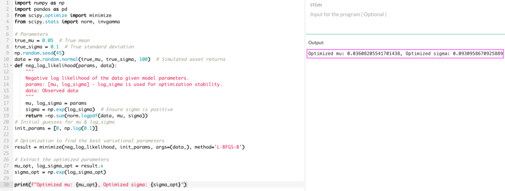
While this simplified approach doesn’t directly compute a full posterior distribution or involve an explicit KL divergence calculation, it gives a basic idea of how one might approach parameter estimation in a Bayesian framework using optimization techniques.

Summary

This example simplifies many aspects of variational Bayesian methods for the sake of accessibility.

In practice, variational inference involves approximating complex posterior distributions by optimizing the parameters of a chosen distribution family to minimize the KL divergence between the approximation and the true posterior.

It often requires more sophisticated techniques and considerations for convergence and accuracy.

Conclusion

Variational Bayesian methods provide a balance between computational efficiency and the ability to model uncertainty.

By providing a probabilistic framework for decision-making, these methods enhance the analysis and management of financial risks, portfolio optimization, algorithmic trading, and other key functions in finance and markets.