Student Loan Debt’s Impact on the Financial Markets

Student loan debt is now close to $2 trillion in the United States, or closing in on 10 percent of GDP.

Student Loans Owned and Securitized, Outstanding

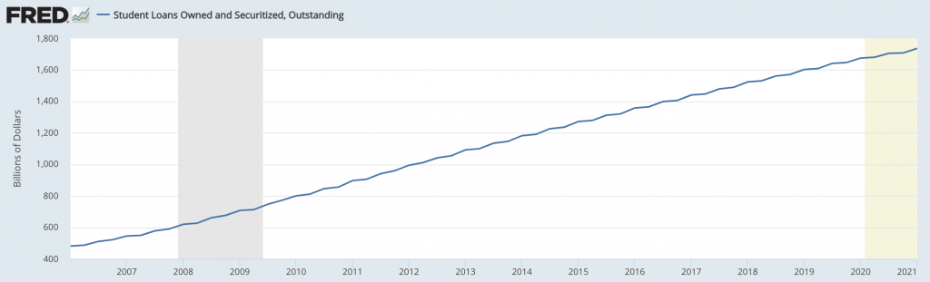
(Source: Board of Governors of the Federal Reserve System (US))

It’s a material line item and it is and will continue to have an impact on money and credit flows throughout the economy and markets. 

How much, if any, of the debt will be relieved by the federal government? 

How much will be defaulted on?

How does that impact consumer behavior? If people owe more money on one thing it means less spending on other things – consumption, housing, stocks and other financial assets. 

Repayments on US federal student loans have come in chronically below expectations. 

The accounting on student loan programs has often been misleading and provided a distorted picture of the actual health of the program.

Congress and various federal administrations have made the student loan program look ostensibly profitable when in reality defaults and losses are more likely. 

If there’s a disparity between what the accounting says and what the loans are genuinely worth, the program will require additional cash infusions from the Treasury. And this would occur long after budgets have already been approved.

The headline national debt would also be larger in reality relative to the current accounting. It could potentially mean hundreds of billions in losses for the federal government.

Current federal government assumptions

The federal government assumes that 96 cents on the dollar will be recovered for every dollar that’s defaulted on.

However, in the private sector, 15-25 cents on the dollar is more common for unsecured credit (i.e., loans not secured with an asset).

How does the government get the near-full recovery amount?

Essentially, the Department of Education puts defaulted borrowers into new loans to cover the old loans. And when the old loans are paid off with the new loans this is considered a “recovery”. 

Nonetheless, in many cases the borrowers have paid down very little to nothing of what they owe, so there’s little to suggest a genuine improvement. They commonly default on the new loans as well because their financial situation hasn’t changed much. 

Recovery is probably more realistically about 50-60 cents on the dollar. 

In the end, of the $2 trillion in total student loans owned and securitized expected by 2025, it could be about a $700 billion hole that will need to be covered. This is beyond the amount lost during the savings and loan crisis of the early 1990s that helped trigger a mild recession.

Implications for the economy

The 2007-09 credit crunch was a function of a lot of defaulted mortgage loans based on flawed assumptions on whether the money could be repaid.

The student loan issue is more mild than the mortgage issue, but $700 billion is still around 3 percent of GDP. 

Whenever there’s a money shortfall, it either takes its effect through incomes (e.g., less spending, less investment, or less savings) or by monetizing it. The first (lower incomes) has bigger effects for the markets and economy, and the second (monetization) has more of an impact on the currency.

If the Congressional Budget Office (CBO), a federal budget watchdog, were to force the federal government to recognize the losses on student loans, the national debt would expand and deficits would deepen. 

The government would also be forced to do something to stem the losses incurred. 

That could mean some type of payment relief. This has been talked about for a long time already, with proponents arguing it could help stimulate the economy by reducing debt burdens.

The Biden Administration has proposed writing off around $10,000 for each student loan borrower. At roughly 43 million borrowers in the US, that comes to around $430 billion total, or almost one-quarter of the total.

Proponents of partial or full relief largely want the government to remain the principal source of the funds.

Critics point to moral hazard, fairness (e.g., people who paid student loans off with their own income and/or savings would not benefit), and other issues. 

Some believe realized losses could force the government to reduce the size of the program. That could prevent some individuals from going to school and picking up the skills and qualifications necessary to become employable to their full potential. 

All budget modeling relies on assumptions and will yield different results. There are many moving parts. 

Like in trading the markets, everything is a distribution with different probabilities associated with various outcomes.

1990 accounting changes

Many of the decisions over the student loan program are based in accounting treatments, which can obscure the underlying fundamentals. 

Before 1990, the federal budget treated student loans as an expense. If the federal government lent out $500 million in student loans, the deficit would rise by an equivalent amount (unless other measures were taken to offset). 

But that law changed in 1990. Future repayments on the loans were now taken into account. 

Now loans become a potential source of profits for the government, assuming that repayments of principal are made with interest and exceed the total cost of defaults. 

Because of the profitability potential, this created the incentive for Congress to expand the program. 

In theory, it would increase access to higher education, increasing the population’s productivity, while potentially providing a profit to the government. 

The projected profits from the program incentivized expansion, as the government believed there would be ROI to actually reduce federal deficits. 

1992 changes

In 1992, the law was changed to enable students from upper-income households to borrow. Interest would also start accumulating when borrowers were still in school rather than after graduation. 

Parents were also now able to borrow more for their children. 

1993 changes

Starting in 1993, income-based repayment plans were established. Instead of a fixed repayment schedule, monthly payments could be spread out over more years – potentially up to 25 rather than just 10. 

This incentivized students to take out larger loans. It also decreased the risk of students not making payments, and thus were seemingly justified to help prevent losses from the program.

2005 changes

In 2005, the burgeoning federal deficit was a concern in both parties. Just five years earlier, there was a budget surplus.

Spending on wars in Afghanistan and Iraq were requiring the largest federal outlays in history. On top of that, as more Baby Boomers were set to hit retirement, more federal outlays would be required in the form of Medicare and Social Security.  

There was a need for more revenue. Tax hikes were unlikely under then-President George W. Bush (a Republican), and tax increases affect capital flows and incentives.

The student loan program was thought to be one way to help pay for it. Either students would be able to more easily afford college and the US would receive a productivity benefit or the returns on the loans would help save the taxpayer’s money. 

Accounting’s impact

The accounting of these measures and assumptions over their impact is largely what led to determinations over their impact on the deficit – and ultimately whether the policy was adopted. Saving money and/or getting a return is always an easy way to help sell an expansion of a program. 

Many projections did come true.

a) Households did borrow more for education.

b) And borrowers were more willing and/or able to pay their loans more when the principal and interest payments were more spread out over time.

Most of those who owed $50,000 or more in student loans to the government had earned graduate degrees. Altogether, more than five million Americans owed that much or more by 2014. 

By 2016, most newly underwritten federal student loans went to graduate students and parents rather than students working on standard four-year degrees. 

However, the assumption that all this new lending would be profitable and return more to the Treasury than it doled out was not consistent with reality.

Over the 16 years from 2002-17, the federal government issued $1.3 trillion in student loans with the expectation that it would return 8 to 9 percent in total ROI (i.e., a bit more than $100 billion in profit). 

But because of new rules and incentives, repayment fell. 

In accordance with those outcomes, government officials revised down their profit expectations to around $70 billion, cutting it by more than one-third. It would have fallen further, but the drop in interest rates enabled the government to fund the loans less expensively. 

The federal government ends its fiscal year at the end of each September. For the 2013 fiscal year (ending in September 2013), it estimated that it would have a net profit of 20 cents for each dollar issued in new student loans. Six years later, that had swung to an expected loss – just 96 cents of every dollar was expected to be recovered. 

The profit assumption underlies whether the program is approved. In the years following, the profit estimates are revised based on the actual repayments that came through. 

If repayments are lower than expected – which is common – the Department of Education gets infused with cash from the Treasury Department. 

This process also takes place outside the purview of Congress and normal budget reviews. Each year the cash infusions required from the Treasury to the Department of Education have grown. 

August 2022 announcement

In August 2022, President Joe Biden announced that $10,000 to $20,000 in federal student debt would be relieved for certain borrowers, subject to income limits and whether the borrower had received Pell Grants.

Skeptics were concerned that the measure wouldn’t get at the root cause of the problem.

The consumer in the federal student loan market is already somewhat price-insensitive because the loans are subsidized and not subject to the standard pricing of credit risk (where the creditor has to consider whether the debt will create enough income to service principal and interest costs).

Wiping out part of the debt creates more of the same agency issue. Losses are borne by the taxpayer and not the colleges and universities, and debt relief could create a consumer that’s even less price-sensitive and incentivize further hikes in tuition and overall cost of attendance.

Worsening fundamentals of the student loan program

Students who took out federal loans in the ten-year 1990-1999 period had repaid about 105 percent of the original balance ten years laters (principal plus some interest). 

However, for the 2006-2015 period, they paid just under 75 percent of the original balance.  

Why are the estimates so far off?

___

Basic credit metrics were ignored

In the federal student loan program, the Department of Education doesn’t look at things like a borrower’s credit score. This is very common in the private sector to help estimate the odds that they’ll repay. Rarely will a private sector lender not pull a prospective borrower’s credit report. 

Based on FI Consulting data, about 40 percent of all student loan borrowers are otherwise “distressed”. For private sector consumer loans, it’s about 20 percent of borrowers.

Nonperforming loans were underestimated

When borrowers default in the student loan program, the government will continue to keep accruing interest on those loans. So balances keep rising. This is typically different from how things work among private lenders, which usually freeze interest payments. 

The governments will generally put these defaulted borrowers into new loans. The interest that accrued will be rolled into the new loan. The borrowers’ loans will then no longer be deemed nonperforming. 

But many of these borrowers also go into default on these new loans, which is why recovery on default is typically quite low and overestimated by the government. 

Income-based repayment may cause principal balances to rise

Borrowers who are unable to make their normal payments also may choose a repayment plan that’s based on income. While such income-based plans are not new, they were expanded under the Obama Administration based on the projection that they wouldn’t expand the deficit. 

The issue with income-based repayment plans is that the interest still accrues. This can cause loan principal balances to rise rather than decline. 

This can make the loans appear more profitable to the government, even though accrual was from the fact that borrowers were having more issues repaying. 

Overestimates of how much borrowers will earn

Department of Education officials might overestimate how much borrowers might earn and therefore how much they’d be able to pay back. 

By law, the DOE cannot look at borrowers’ tax statements to gain an understanding of repayment ability, as private lenders might require. 

When the loans reach the end of their repayment cycle, about one-third of the balance would end up at the taxpayer’s expense. 

This could potentially cause the government to need to come up with hundreds of billions of new cash to help balance the books.

The OMB has final say

The Office of Management and Budget (OMB) uses data from the Department of Education to estimate how much federal student loans will either earn a profit or loss. 

The OMB ultimately dictates how the accounting is handled for purposes of the federal budget process. 

The projected profits used for accounting purposes don’t help make changes that could be beneficial for both the government and borrowers. Lower interest rates could help borrowers pay back the loans and help the government’s ultimate recovery. 

This is particularly true given the government’s projected profits are too high.  

Despite low interest rates – zero to two percent range on US Treasury bonds (where the US government can borrow at) – many loans are still north of seven percent. 

Graduate and parent loans tend to come with a higher interest rate than those for undergraduates. 

Per law, federal student loans also can’t be refinanced at lower interest rates by the Department of Education. Borrowers with high interest rates on their federal student loan debt are stuck with those rates unless they obtain cheaper private loans. 

When borrowers do get private loans to pay off their federal student loans, the government loses out on interest it could have earned. In turn, this means the government’s portfolio ends up weighted more toward borrowers that are less likely to repay their loans. 

This could be from the fact that they:

• Didn’t graduate and couldn’t put any degree to use
• Have jobs that don’t pay well enough
• Borrowed too much money that they can’t repay

Market implications

Governments are the biggest influence on money and credit flows. 

In developed markets, interest rates are low across the yield curve, from short-term (cash) to long-term bonds. This means traditional policies from central banks – i.e., adjustment of short-term interest rates and QE (asset buying) – no longer work as well. 

More of the control over the economy will come from the fiscal side, which is controlled by the politicians. 

As the student loan program has grown into around 10 percent of GDP, it’s a material part of the budget. 

It has an impact on virtually everything in some way. 

If each student loan borrower was given $10,000 to pay off their loans, how would that flow through the economy and markets? That’s nearly $500 billion. 

Any type of relief would be viewed as a positive for:

• Stocks (more money to put to use in the stock market and other traditional financial assets)
• Real estate
• Commodities (more demand)
• Gold (money would need to be created, which is a negative for the dollar, and positive for alternative stores of value)

And negative for:

• The dollar (more money needs to be created)
• Bonds (more bond issuance with weak demand for it, given low/negative real rates)

The student loan program is also a source of tail risk. The extra indebtedness consumers face (without deriving income in excess of the debt on net) creates a more tenuous financial situation for tens of millions of Americans. 

And the situation is likely to worsen. Accordingly, it will require more oversight by the government. Increasing cash infusions from the Treasury Department to the Department of Education are likely. 

As the debt burden swells, it will also become more politically popular to consider a combination of write-offs from the government (i.e., giving each borrower a certain amount to apply to loan servicing) or more stringent underwriting standards.