Stochastic Portfolio Theory & Chance-Constrained Portfolio Selection

Stochastic Portfolio Theory (SPT) is a mathematical framework used to analyze and manage portfolios of assets in probabilistic terms.

It extends the classical Markowitz portfolio theory by incorporating the randomness inherent in financial markets.

Key Takeaways – Stochastic Portfolio Theory & Chance-Constrained Portfolio Selection

• Stochastic Portfolio Theory (SPT) focuses on understanding and exploiting patterns in the stochastic behavior of assets to optimize portfolio construction.
  • Emphasizes the role of randomness in markets and the fact that they’re not deterministic. (One needs to be comfortable with the fact that markets are an applied probability exercise.)
• Chance-Constrained Portfolio Selection integrates probabilistic constraints.
  • Allows traders/investors to specify acceptable risk levels in terms of probabilities – i.e., directly incorporating uncertainty into portfolio optimization.
• This approach enables more robust risk management by quantifying and limiting potential losses, such as drawdowns or underperformance, under specified confidence levels.
  • Improves on traditional models with a realistic assessment of uncertainty.

Foundations of Stochastic Portfolio Theory

SPT was developed to provide a more realistic approach to portfolio management.

Unlike traditional models, which often rely on fixed or historical data, SPT considers the uncertain nature of asset returns.

It uses stochastic processes to model asset price dynamics.

It acknowledges that future asset prices are not deterministic but subject to random fluctuations.

Key Principles

Randomness in Asset Returns

SPT treats asset returns as random variables.

This approach allows for the modeling of real-world phenomena like volatility clustering and fat-tailed distributions of returns.

Dynamic Portfolio Management

SPT emphasizes a dynamic view of portfolio management, where asset allocations are continuously adjusted.

Diversification Benefits

The theory underlines the importance of diversification, not just in terms of asset types but also in the strategies used to manage them.

Chance-Constrained Portfolio Selection

Chance-constrained portfolio selection is a specific application within SPT.

In a typical portfolio optimization, a trader might want to maximize expected returns subject to a maximum acceptable level of risk.

However, risk and return estimations are uncertain due to the stochastic nature of financial markets.

Chance constraints tackle this by allowing the investor to specify acceptable levels of risk in probabilistic terms.

Example – No more than a 20% drawdown in a portfolio

In the context of chance-constrained portfolio selection, a trader aiming to limit drawdowns to less than 20% is essentially focusing on controlling the maximum loss from peak to trough in the portfolio’s value.

This constraint can be formulated probabilistically to manage risk under uncertainty.

Let’s define a drawdown constraint in a chance-constrained framework.

Suppose a trader specifies that the portfolio should not experience more than a 20% drawdown with a 95% confidence level.

Mathematically, this can be represented as:

P (D ≤ 20%) ≥ 95%

Here, D represents the drawdown, and the constraint ensures that the probability of the drawdown exceeding 20% is no more than 5% (i.e., the complement of the 95% confidence level).

To implement, the trader would use historical data, statistical models, or simulations like Monte Carlo methods to estimate the distribution of potential portfolio drawdowns.

For example, in other articles, we’ve covered Monte Carlo simulations as it pertains to calculating VaR.

These methods take into account the correlations and volatilities of the individual assets, as well as the macroeconomic factors (e.g., changes in discounted growth and discounted inflation) influencing their returns.

The portfolio is then optimized by selecting weights of different assets that minimize the expected drawdown or ensure that the probability of exceeding the 20% threshold remains below the specified level.

For example, a Monte Carlo simulation might be used to generate a wide range of possible portfolio paths based on historical returns and volatilities.

The drawdown for each simulated path is calculated, and the proportion of paths where the drawdown exceeds 20% is determined.

The portfolio weights are then adjusted iteratively in the optimization algorithm to ensure that this proportion is less than or equal to 5%, adhering to the trader’s risk appetite.

Accordingly, by using chance-constrained portfolio selection with a focus on limiting drawdowns, traders can balance the trade-off between portfolio performance and the risk of significant losses.

This approach provides a structured way to incorporate risk management directly into the portfolio construction process, and will cater to the specific risk tolerance and objectives of the trader.

Concept and Application

Risk Constraints

Instead of setting fixed constraints (like a maximum drawdown limit), chance-constrained models define constraints in terms of probabilities.

For example, a constraint might limit the probability of a portfolio’s return falling below a certain threshold.

Optimization Problem

The central task is to maximize expected returns while ensuring that the chance constraints are satisfied.

This involves balancing the trade-off between risk and return in a probabilistic setting.

Mathematical Formulation

Objective Function

Typically, the objective function in a chance-constrained portfolio model aims to maximize expected returns or utility.

Constraints

Constraints are formulated as inequalities that incorporate probability measures.

For instance, a constraint might be that the probability of returns being less than -5% should be less than 10%.

Solving the Model

Solving chance-constrained problems often requires optimization techniques and numerical methods.

Python Coding Example

Let’s assume we have this portfolio with the following characteristics:

• 40% Stocks: +6% forward return, 15% annualized volatility using standard deviation
• 45% Bonds: +4% forward return, 10% annualized volatility using standard deviation
• 5% Commodities: +3% forward return, 15% annualized volatility using standard deviation
• 10% Gold: +3% forward return, 15% annualized volatility using standard deviation

Assume a 0% correlation between assets.

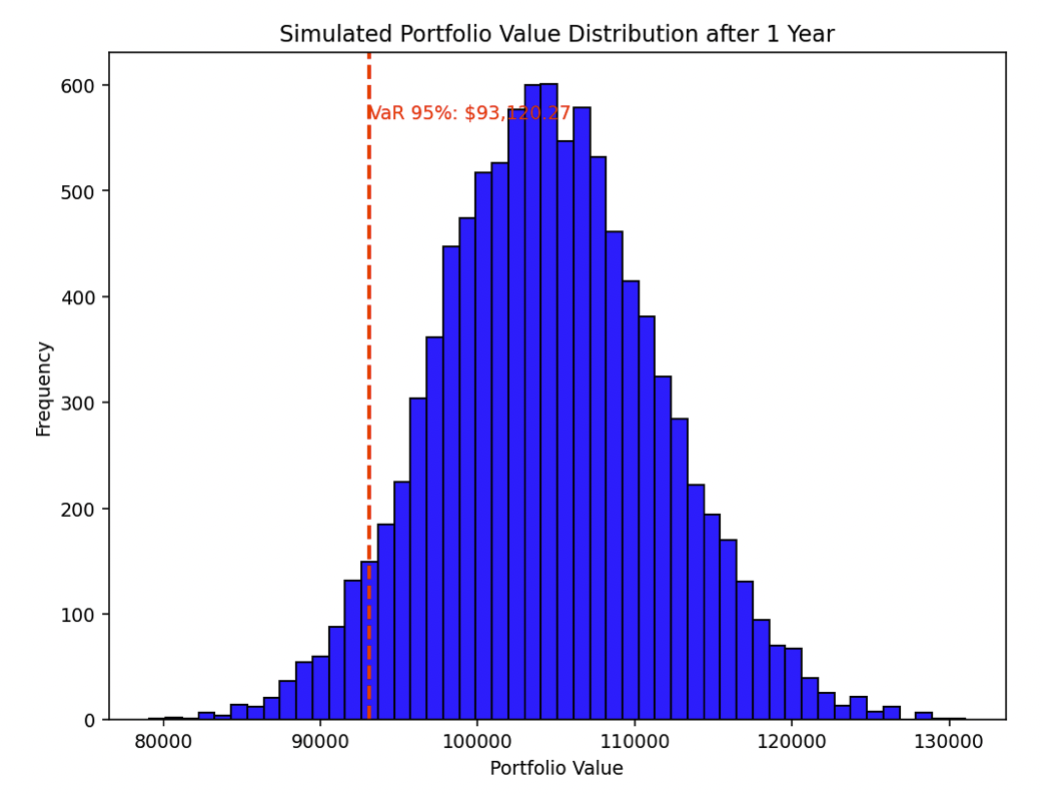
And let’s say we understand that markets are stochastic and want to plot a Monte Carlo diagram.

Then we want to calculate the 99% VaR.

Here’s how we can do it with code:

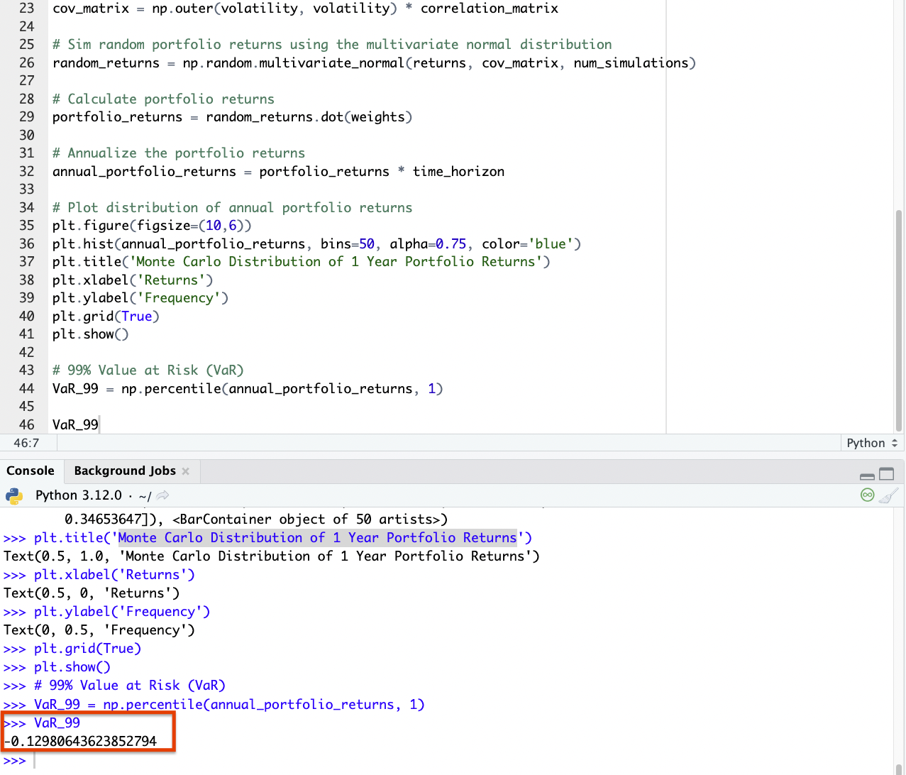
import numpy as np

import matplotlib.pyplot as plt

# Portfolio weights

weights = np.array([0.4, 0.45, 0.05, 0.1])

# Expected forward returns

returns = np.array([0.06, 0.04, 0.03, 0.03])

# Annualized volatility (standard deviation)

volatility = np.array([0.15, 0.10, 0.15, 0.15])

# Correlation matrix (0% correlation between assets)

correlation_matrix = np.eye(4)  # Identity matrix for 0% correlation

# Number of simulations

num_simulations = 10000

# Time horizon in years for the simulation

time_horizon = 1

# Convert the correlation matrix to a covariance matrix

cov_matrix = np.outer(volatility, volatility) * correlation_matrix

# Sim random portfolio returns using the multivariate normal distribution

random_returns = np.random.multivariate_normal(returns, cov_matrix, num_simulations)

# Calculate portfolio returns

portfolio_returns = random_returns.dot(weights)

# Annualize the portfolio returns

annual_portfolio_returns = portfolio_returns * time_horizon

# Plot distribution of annual portfolio returns

plt.figure(figsize=(10,6))

plt.hist(annual_portfolio_returns, bins=50, alpha=0.75, color='blue')

plt.title('Monte Carlo Distribution of 1 Year Portfolio Returns')

plt.xlabel('Returns')

plt.ylabel('Frequency')

plt.grid(True)

plt.show()

# 99% Value at Risk (VaR)

VaR_99 = np.percentile(annual_portfolio_returns, 1)

VaR_99

Here’s our diagram:

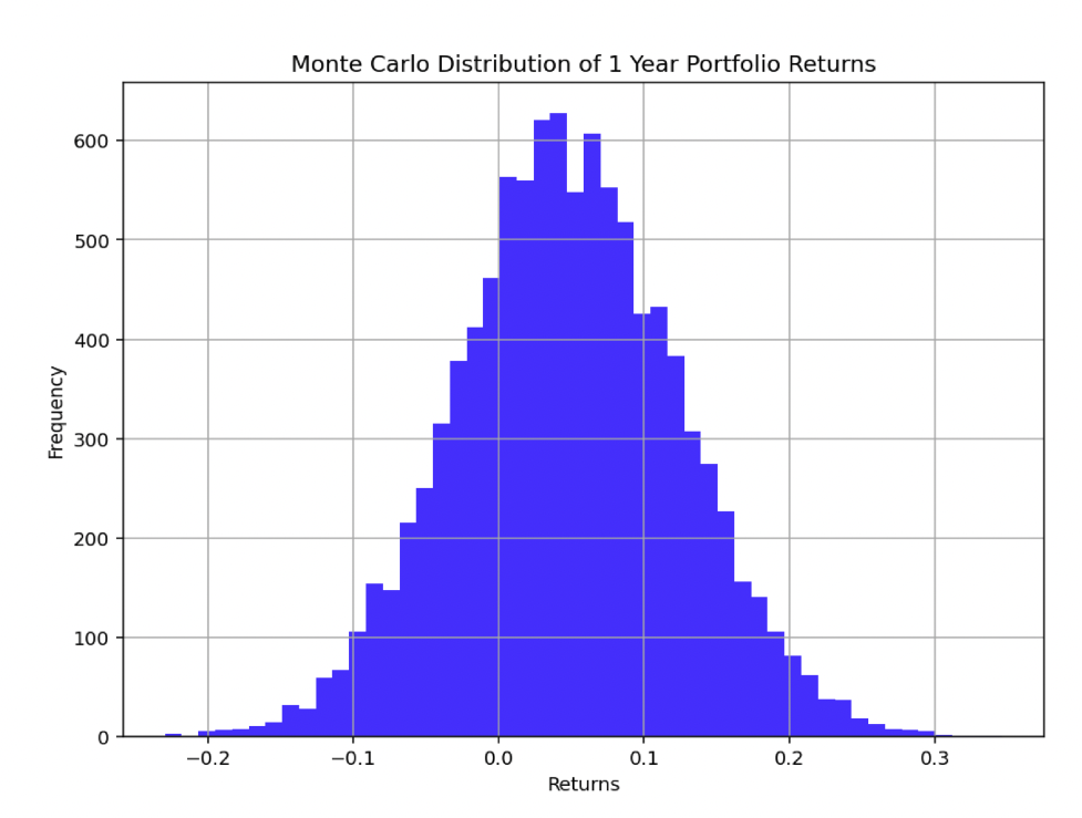
And we find that our 99% VaR is about a 13% loss.

If we wanted to find this portfolio’s average returns, we could simply run these lines:

Returns_avg = np.percentile(annual_portfolio_returns, 50) 

Returns_avg

And from this, we get 4.6%.

And about 70-75% of the years, this portfolio would make money.

Importance in Modern Finance

Realistic Risk Assessment

Chance-constrained portfolio selection provides a more nuanced and realistic approach to risk management.

It acknowledges that markets will move in ways that can’t be anticipated.

Adaptability

It allows for more flexible and adaptive portfolio strategies, which are essential in rapidly changing market environments.

Advanced Risk Measures

This approach facilitates the use of risk measures like Value at Risk (VaR) and Conditional Value at Risk (CVaR).

Conclusion

Stochastic Portfolio Theory and chance-constrained portfolio selection offer a more realistic and adaptable framework for managing portfolios, given the stochastic nature of financial markets.

These methods are valuable for traders, investors, and portfolio managers seeking to optimize returns while effectively managing risk in a probabilistic context.