How to Design an Algorithm for Predicting Exchange Rates

Designing an algorithm for predicting exchange rates involves a series of steps that integrates knowledge in finance, economics, math, programming, and machine learning.

Key Takeaways – How to Design an Algorithm for Predicting Exchange Rates

• Incorporate Relevant Variables:
  • Include key macroeconomic indicators like interest rates, inflation, GDP, and political stability, as they all influence exchange rates.
  • (What you included depends on your strategy.)
• Employ Advanced Statistical Models:
  • Use time series analysis, machine learning algorithms, and econometric models to capture complex relationships in financial data.
• Rigorous Validation and Testing:
  • Implement robust backtesting and validation strategies to ensure the algorithm’s accuracy and reliability in different market conditions.
• Example Model:
  • We give an example at the bottom of this article of a type of approach using synthetic data.

Here’s an outline of the process:

Define the Objective

Clearly articulate the goal of the algorithm.

Is it to predict short-term fluctuations or long-term trends in exchange rates?

Understanding the trading, investment, or operational horizon is important.

Gather and Preprocess Data

Data Sources

Identify and collect relevant data.

This includes historical exchange rates, macroeconomic indicators (like GDP, inflation rates, interest rates), political events, and market sentiment data.

Data Cleaning

Address missing values, outliers, and inconsistencies in the data.

Feature Engineering

Create new features that could be relevant for the prediction, such as moving averages, lagged variables, or indicators derived from text data (e.g., sentiment analysis of news articles).

Exploratory Data Analysis (EDA)

Analyze the data to uncover patterns, trends, and correlations.

Use visualizations to understand the relationships between variables.

Perform statistical tests to validate hypotheses about the data.

Model Selection

Choose appropriate models based on the nature of the data and the prediction goal.

Options include linear regression models, time series models (like ARIMA), machine learning algorithms (such as Random Forest, SVM, neural networks), and advanced techniques like LSTM (Long Short-Term Memory) networks for sequence prediction.

Feature Selection and Dimensionality Reduction

Identify the most relevant features for the model.

Apply techniques like PCA (Principal Component Analysis) for dimensionality reduction if needed.

Model Training and Validation

Split the data into training and testing sets.

Train the model on the training set and validate its performance on the testing set.

Use metrics like RMSE (Root Mean Square Error), MAE (Mean Absolute Error), and AIC (Akaike Information Criterion) for model evaluation.

Hyperparameter Tuning

Optimize the model by tuning its hyperparameters.

Use methods like grid search or random search to find the optimal set of hyperparameters.

Backtesting

Test the model’s performance against historical data – i.e., backtesting.

Ensure that the model is robust and performs well across different time periods and market conditions.

Incorporate Risk Management Strategies

Include measures to account for model risk, market risk, and other financial risks.

Implement strategies like position exiting or position sizing based on the model’s confidence intervals.

Deployment

Integrate the model into the desired platform for real-time or batch processing.

Ensure the model has access to real-time data feeds for live predictions.

Monitoring and Updating

Continuously monitor the model’s performance.

Update the model regularly with new data and adjust the model as market conditions change or you think of new, relevant criteria to test.

Documentation and Compliance

Thoroughly document the model, including its design, data sources, assumptions, and limitations.

Ensure the model complies with relevant regulatory and ethical standards.

Examples of Variables to Include

Focusing on macroeconomic variables for predicting exchange rates involves a careful selection of indicators that can influence currency value.

Here’s a list of key macroeconomic variables that you should consider integrating into your model (if you choose to pursue this longer-term fundamental approach):

Interest Rates

Central banks influence exchange rates through their control of interest rates.

Higher interest rates offer lenders a higher return relative to other countries, attracting foreign capital and causing the exchange rate to rise.

Inflation Rates

Generally, countries with consistently low inflation rates exhibit a rising currency value, as their purchasing power increases relative to other currencies.

Conversely, higher inflation typically depreciates the value of a currency in relation to the currencies of its trading partners.

Gross Domestic Product (GDP)

The GDP is a primary indicator of the economic health of a country.

A high GDP growth rate often strengthens the respective country’s currency as it implies a robust economy.

Current Account Balance

The current account reflects the country’s balance of trade, earnings on foreign investment, and cash transfers.

A current account surplus indicates that the country is a net lender to the rest of the world, which can strengthen its currency.

Government Debt

Countries with large amounts of debt are less likely to attract foreign investment, leading to a decrease in currency value.

High debt may prompt inflation – i.e., rising debt loads, which may be unwanted and lead to higher interest rates to help clear the market – which can depreciate the currency.

Political Stability and Economic Performance

Countries that are politically stable and have strong economic performance tend to attract foreign investors.

Political and economic stability influence foreign investors’ confidence, impacting the currency value.

Terms of Trade

Changes in export and import prices impact the terms of trade.

If the price of a country’s exports rises compared to its imports, its terms of trade have improved, increasing revenue and causing a rise in the value of its currency.

Employment Indicators

Employment levels in an economy affect consumer spending and economic growth.

Higher employment typically leads to a stronger economy and potentially a stronger currency.

Monetary Policy Statements

Central bank communications and policy statements can have immediate effects on currency markets, as they often contain hints about future monetary policy.

Foreign Exchange Reserves

The amount of a currency held in reserves by foreign governments can affect currency value.

Large reserves of foreign currency can be used to stabilize the domestic currency.

Capital Flows

This includes Foreign Direct Investment (FDI) and Portfolio Investment.

The flow of capital into and out of a country can influence exchange rates as they change the demand for the domestic currency.

Global Economic Indicators

Since the economy is globally interconnected, international economic indicators can also impact exchange rates.

This includes economic health indicators from major trading partners or global economic entities like the European Union, China, or the United States.

Summary

Incorporating these variables into your model involves careful data collection, preprocessing, and analysis.

The relationship between these variables and exchange rates can be complex and non-linear.

This may require advanced statistical techniques and machine learning algorithms for accurate modeling and prediction.

Additionally, the significance and impact of each variable may vary depending on the specific currency pair and the economic context being analyzed.

Mathematical, Statistical, and Algorithmic Methods

For predicting exchange rates using macroeconomic variables, a blend of mathematical, statistical, and algorithmic techniques can be employed.

Given the complexity and dynamic nature of financial markets, it’s essential to use sophisticated methods that can capture the intricate relationships between different variables and their impact on exchange rates.

Here are some key techniques:

Time Series Analysis

ARIMA (Autoregressive Integrated Moving Average)

Useful for modeling time series data, particularly for forecasting based on historical data.

VAR (Vector Autoregression)

A generalization of ARIMA that can model interdependencies between multiple time series (e.g., different macroeconomic indicators).

GARCH (Generalized Autoregressive Conditional Heteroskedasticity)

Effective in modeling financial time series that exhibit volatility clustering, a common trait in exchange rate data (and generally all asset data).

Machine Learning Algorithms

Random Forest

An ensemble learning method for classification and regression that can handle a large number of features and identify important variables.

Support Vector Machines (SVM)

Effective in high-dimensional spaces, SVMs are good for datasets where the number of dimensions exceeds the number of samples.

Neural Networks and Deep Learning

Especially LSTM (Long Short-Term Memory) networks, which are adept at capturing long-term dependencies in time series data.

Econometric Models

Cointegration Analysis

This tests for a long-term equilibrium relationship between exchange rates and macroeconomic variables.

Panel Data Models

If you’re analyzing data that spans across different countries or time periods, panel data models like Fixed Effects or Random Effects models can be useful.

Statistical Techniques

Principal Component Analysis (PCA)

For dimensionality reduction and to identify underlying factors that explain the variance in exchange rates.

Granger Causality Tests

To test whether one time series can predict another.

This is important in establishing relationships between macroeconomic variables and exchange rates.

Bayesian Methods

Bayesian Regression Models

Useful when dealing with small datasets or when incorporating prior beliefs or information into the analysis.

Markov Chain Monte Carlo (MCMC)

For complex models where traditional inference is difficult, MCMC provides methods for sampling from probability distributions.

Optimization Techniques

Gradient Descent and its Variants (e.g., Stochastic Gradient Descent)

For optimizing the parameters of machine learning models, especially neural networks.

Genetic Algorithms

Useful for optimizing feature selection and model parameters in complex, non-linear problems.

Related: Heuristic & Metaheuristic Methods

Regularization Methods

Ridge Regression (L2 Regularization)

To prevent overfitting by penalizing large coefficients.

Lasso Regression (L1 Regularization)

Useful for feature selection as it can shrink coefficients of less important variables to zero.

Sentiment Analysis and Natural Language Processing (NLP)

To incorporate qualitative data from news articles, reports, or social media, which can have an impact on exchange rates.

Summary

Each of these techniques offers distinct advantages and can be chosen based on the specific characteristics of your dataset, the complexity of the model, and the prediction goals.

Often, a hybrid approach that combines multiple techniques can yield better results.

At the very least, it can help you triangulate.

Example Algorithm

Creating a complete exchange rate prediction model involves several steps, including data gathering, preprocessing, feature selection, model building, and evaluation.

This example assumes you have a dataset with historical exchange rates and corresponding macroeconomic variables.

We’ll use a machine learning approach with a Random Forest regressor for this example.

Part 1: Import Libraries and Load Data

import pandas as pd
import numpy as np
from sklearn.model_selection import train_test_split
from sklearn.ensemble import RandomForestRegressor
from sklearn.metrics import mean_squared_error
import matplotlib.pyplot as plt

# Load your dataset, which should contain historical exchange rates and macroeconomic variables
# Replace 'your_dataset.csv' with your actual dataset file
data = pd.read_csv('your_dataset.csv')

Part 2: Data Preprocessing

# Assuming the dataset has columns like 'exchange_rate', 'interest_rate', 'inflation_rate', etc.
# Check for missing values
data = data.dropna()

# Separate the features and the target variable
X = data.drop('exchange_rate', axis=1) # Features (Macroeconomic Variables)
y = data['exchange_rate'] # Target Variable

# Split the dataset into training and testing sets
X_train, X_test, y_train, y_test = train_test_split(X, y, test_size=0.2, random_state=42)

Part 3: Model Building

# Start the Random Forest Regressor
rf_model = RandomForestRegressor(n_estimators=100, random_state=42)

# Train the model
rf_model.fit(X_train, y_train)

Part 4: Model Evaluation

# Predicting the Exchange Rates
y_pred = rf_model.predict(X_test)

# Calculate the Mean Squared Error
mse = mean_squared_error(y_test, y_pred)
print(f"Mean Squared Error: {mse}")

# Plot Predicted vs Actual Values
plt.scatter(y_test, y_pred)
plt.xlabel('Actual Exchange Rates')
plt.ylabel('Predicted Exchange Rates')
plt.title('Predicted vs Actual Exchange Rates')
plt.show()

Since this example is a bit abstract without the data, let’s design one with synthetic data and include the macro variables we covered above:

# Set random seed
np.random.seed(55)

# Number of samples
n_samples = 1000

# Generating synthetic features
interest_rates = np.random.normal(2, 0.5, n_samples) # Interest Rates
inflation_rates = np.random.normal(2, 1, n_samples) # Inflation Rates
gdp_growth = np.random.normal(3, 1, n_samples) # GDP Growth
current_account_balance = np.random.normal(0, 1, n_samples) # Current Account Balance
government_debt = np.random.normal(50, 10, n_samples) # Government Debt
political_stability = np.random.choice([0, 1], size=n_samples, p=[0.3, 0.7]) # Political Stability (0: unstable, 1: stable)
terms_of_trade = np.random.normal(100, 20, n_samples) # Terms of Trade
employment_rate = np.random.normal(5, 1, n_samples) # Employment Rate
monetary_policy_statements = np.random.choice([0, 1, 2], size=n_samples, p=[0.3, 0.4, 0.3]) # Monetary Policy (0: tightening, 1: neutral, 2: loosening)
foreign_exchange_reserves = np.random.normal(100, 25, n_samples) # Foreign Exchange Reserves
capital_flows = np.random.normal(0, 1, n_samples) # Capital Flows

# Generating synthetic target variable (Exchange Rate)
# The formula used here is hypothetical and for illustrative purposes
exchange_rates = 50 + 1.5*interest_rates - 2*inflation_rates + 1.2*gdp_growth + 0.5*current_account_balance - \
0.3*government_debt + 2*political_stability + 0.1*terms_of_trade - 0.5*employment_rate + \
0.4*monetary_policy_statements + 0.2*foreign_exchange_reserves + 0.3*capital_flows + \
np.random.normal(0, 2, n_samples)

# Creating the DataFrame
data = pd.DataFrame({
'Interest Rates': interest_rates,
'Inflation Rates': inflation_rates,
'GDP Growth': gdp_growth,
'Current Account Balance': current_account_balance,
'Government Debt': government_debt,
'Political Stability': political_stability,
'Terms of Trade': terms_of_trade,
'Employment Rate': employment_rate,
'Monetary Policy Statements': monetary_policy_statements,
'Foreign Exchange Reserves': foreign_exchange_reserves,
'Capital Flows': capital_flows,
'Exchange Rates': exchange_rates
})

# Splitting the dataset
X = data.drop('Exchange Rates', axis=1)
y = data['Exchange Rates']
X_train, X_test, y_train, y_test = train_test_split(X, y, test_size=0.2, random_state=10)

# Building the Random Forest model
rf_model = RandomForestRegressor(n_estimators=100, random_state=10)
rf_model.fit(X_train, y_train)

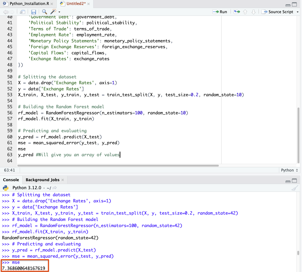
# Predicting and evaluating
y_pred = rf_model.predict(X_test)
mse = mean_squared_error(y_test, y_pred)
mse

y_pred #Will give you an array of values

From this, we see that this Random Forest model, trained on a synthetic dataset incorporating a wide range of macroeconomic variables, yields a Mean Squared Error (MSE) of approximately 7.76.

This value represents the average squared difference between the actual and predicted exchange rates in our synthetic dataset.

This is reasonable considering the exchange rate tends to hover between 50-80 and based on the number of variables in our model.

How close did the predicted exchange rates match the actual exchange rate?

We can make a graph for this:

plt.figure(figsize=(10, 6))

# Actual vs Predicted
plt.scatter(range(len(plot_data)), plot_data['Actual'], label='Actual Exchange Rates', color='red', alpha=0.7)
plt.scatter(range(len(plot_data)), plot_data['Predicted'], label='Predicted Exchange Rates', color='blue', alpha=0.7)

# Confidence Interval
plt.fill_between(range(len(plot_data)), plot_data['Lower Bound'], plot_data['Upper Bound'], color='skyblue', alpha=0.4)

# Adding titles and labels
plt.title('Exchange Rate Prediction with Confidence Intervals')
plt.xlabel('Data Points')
plt.ylabel('Exchange Rate')
plt.legend()
plt.show()

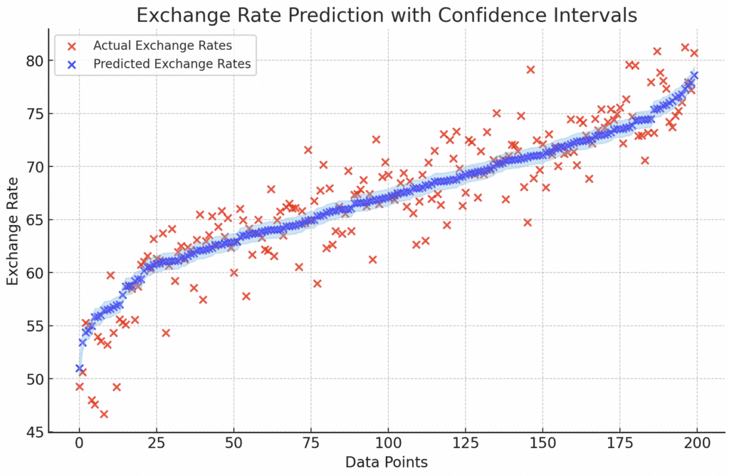
The graph uses blue dots to represent the predicted exchange rates and red dots for the actual exchange rates. 

The blue cloud around the predictions illustrates the confidence intervals.

This visualization compares each predicted exchange rate with the corresponding actual rate. 

The proximity of the blue dots to the red dots indicates how close the predictions are to the actual values. 

The confidence interval (blue cloud) provides insight into the uncertainty or variability around each prediction.

Machine Learning Models for Currency Trading Systems & Hidden Variable Detection

Currency trading is complex because there are so many variables and it’s hard to capture everything.

And the weights of each differ.

For example, remittances have bigger effects on the exchange rates of EM currencies than they do on reserve currencies like the USD.

For enhancing the prediction of currency values and identifying hidden variables in financial data, several advanced machine learning techniques can be leveraged beyond the basic unsupervised learning methods like clustering and principal component analysis (PCA).

These techniques are designed to handle the complexity and non-linearity of financial markets:

Supervised Learning

Regression Analysis

Advanced regression techniques, such as Ridge, Lasso, and Elastic Net, can be used for feature selection and regularization to handle multicollinearity and overfitting while identifying the most influential variables.

Decision Trees and Random Forests

These can be used for both classification and regression tasks.

Random forests, an ensemble of decision trees, are good at capturing nonlinear relationships and interactions between variables.

Unsupervised Learning

Autoencoders

A type of neural network used for unsupervised learning of efficient codings.

Autoencoders can help identify complex, nonlinear relationships in the data and potentially suggest hidden variables through the reconstruction error.

t-Distributed Stochastic Neighbor Embedding (t-SNE)

This technique is useful for visualizing high-dimensional data in lower-dimensional spaces, which can help in identifying clusters or patterns that suggest missing variables.

Semi-Supervised Learning

Techniques that leverage both labeled and unlabeled data can be particularly useful when there’s a limited amount of labeled data available.

This approach can help in identifying underlying structures or patterns that are not evident when using only labeled or only unlabeled data.

Reinforcement Learning

Although traditionally used for decision-making processes, reinforcement learning can also be applied to identify strategies that could predict currency values effectively.

It can work to adapt to new data and potentially uncover hidden variables through exploration.

Deep Learning

Convolutional Neural Networks (CNNs)

Primarily used for image processing, CNNs can also be applied to time-series data to capture spatial hierarchies in data and identify complex patterns over time.

Recurrent Neural Networks (RNNs) and Long Short-Term Memory Networks (LSTMs)

These are particularly suited for sequential data like time series, capable of learning long-term dependencies and identifying patterns that simpler models might miss.

Graph Neural Networks (GNNs)

For financial data structured as graphs (e.g., interbank lending networks), GNNs can capture the relationships and interactions between entities, potentially uncovering hidden variables influencing currency values.

Bayesian Methods

Gaussian Processes

These can be used for regression and classification tasks, which offer a probabilistic approach to learning.

Gaussian processes are beneficial for modeling uncertainty, which can help in identifying when new, unconsidered variables might be influencing predictions.

Ensemble Methods

Boosting (e.g., XGBoost, LightGBM, AdaBoost)

These techniques combine multiple weak learners to create a strong predictive model.

They are useful for improving model performance and stability, and could highlight which features (variables) contribute most to predicting currency values.

Summary

Each of these techniques has its strengths and can be particularly suited to different aspects of financial data analysis.

The choice of technique would depend on the:

• specific characteristics of the data
• computational resources available, and
• complexity of the relationships between variables in predicting currency values

Conclusion

This algorithm, when designed well and rigorously tested, can serve as a tool in predicting exchange rates.

It can help in strategic decision-making for financial institutions, traders, and policymakers.