Conic Solvers in Financial Optimization Problems (Applications & Python Example)


Conic solvers are used in financial optimization, where accuracy and computational efficiency are most important.
Financial optimization involves the use of mathematical models to make optimal decisions regarding trading and investment decisions and risk management.
This field often requires dealing with complex constraints and objectives.
This is where conic solvers come into play.
Key Takeaways – Conic Solvers in Financial Optimization Problems
- Efficient for Convex Problems: Conic solvers efficiently handle convex optimization problems common in finance.
- Ensures accurate, globally optimal solutions.
- Complex Constraint Management: They excel in incorporating complex financial constraints into optimization models (e.g., risk limits, regulatory requirements).
- Versatile Applications: Widely used in financial optimization tasks like portfolio management, risk assessment, and asset pricing due to their robustness and precision.
- Python Example: We do an example of a conic solver optimization using a simple 3-asset portfolio.
1. The Role of Conic Solvers in Financial Optimization
Nature of Conic Programming
Conic programming is a subset of convex optimization where the feasible region is defined by a convex cone.
A convex cone is a set that is closed under positive scaling and addition, which includes linear, quadratic, and semidefinite programming problems.
Complex Financial Models
In finance, models often incorporate various types of risks and return objectives that can be formulated as convex problems.
This can include mean and variance (i.e., return and risk), and “higher moments” like skewness and kurtosis, which have to do with the shape of the distribution of returns.
Conic solvers are good at handling these complexities efficiently.
2. Types of Conic Solvers in Finance
Linear Solvers
Used for portfolio optimization and asset allocation where the constraints and objectives are linear.
Quadratic Solvers
Applicable in mean-variance optimization and in the modeling of quadratic utility functions.
Semidefinite Solvers
Employed in advanced risk modeling, including correlation and covariance matrix estimation under uncertainty.
3. Applications in Financial Optimization
Portfolio Optimization
Adjusting the weights of assets in a portfolio to maximize return for a given level of risk, or vice versa.
Risk Management
Quantifying and managing financial risks, such as market risk, credit risk, and operational risk.
Often has complex interdependencies.
Asset Pricing
Developing models to accurately price financial derivatives.
Takes into account various factors like volatility and correlation.
Related: Options Pricing Models
4. Advantages of Using Conic Solvers
Robustness and Efficiency
Conic solvers are known for their robustness and ability to efficiently handle large-scale problems with high-dimensional data.
Handling Nonlinearities and Unknowns
They are particularly useful in dealing with nonlinear relationships and unknowns inherent in financial data.
Accurate Risk Assessment
Conic solvers provide precise solutions to complex optimization problems.
5. Challenges and Considerations
Model Specification and Parameterization
Accurate model specification is important.
Incorrect assumptions or misestimation of parameters can lead to suboptimal solutions.
Related: Non-Parametric Models in Finance
Computational Complexity
Some conic problems (e.g., large-scale semidefinite programs) can be computationally intensive.
Data Quality and Availability
The effectiveness of these solvers is contingent on the quality and availability of financial data.
6. Future Trends and Developments
Integration with Machine Learning
Leveraging machine learning techniques for dynamic model parameterization and prediction of financial variables.
More optimization work is moving toward machine learning and automation.
Advancements in Algorithm Efficiency
Continuous research in improving the computational efficiency of conic solvers – especially for large-scale problems.
Broader Application Areas
Expanding the use of conic solvers to newer areas in finance.
Why would you use conic solvers for optimization versus other approaches?
Using conic solvers for optimization in financial contexts – as opposed to other approaches – is driven by several factors:
Handling of Convex Problems
Nature of Financial Optimization Problems
Many optimization problems in finance are naturally convex (meaning they have a single global minimum).
Conic solvers are specifically designed for convex problems.
This ensures global optimality.
Robustness in Convex Settings
They provide robust solutions in convex settings.
This is important in finance where even small errors can result in financial repercussions.
Efficiency in High-Dimensional Spaces
Scalability
Conic solvers efficiently handle high-dimensional problems common in finance.
This includes:
- large portfolio optimizations (i.e., portfolios with lots of different assets or active trades) or
- risk management scenarios involving numerous variables and constraints
Speed
They often offer superior computational speed.
This is important in finance where decisions need to be made rapidly – in many cases, in near real-time.
Versatility and Flexibility
Wide Range of Problem Types
Conic solvers can address various forms of convex problems, such as linear, quadratic, and semidefinite programming.
This versatility is valuable in finance where different problems require different approaches.
Incorporation of Complex Constraints
Financial models often involve complex constraints.
This includes regulatory requirements, risk limits, and transaction costs.
Conic solvers excel at incorporating and efficiently solving problems with such constraints.
Precision and Accuracy
Exact Solutions for Convex Problems
They are known for providing precise and accurate solutions for convex optimization problems.
Stability in Solutions
Conic solvers offer stable solutions even in the presence of data uncertainties and model perturbations, a common scenario in financial markets.
Risk Management Capabilities
Conic solvers are good at handling optimization problems involving risk measures like Value at Risk (VaR) or Conditional Value at Risk (CVaR).
These are nonlinear and can be modeled as convex optimization problems.
Theoretical Foundations
They are grounded in solid mathematical theory.
This provides a level of assurance in the integrity of the solutions.
Comparison with Other Methods
Non-Convex Solvers
While there are solvers for non-convex problems, they often don’t guarantee global optimality and can be trapped in local minima (less desirable in financial decision-making).
(If these terms are confusing, we have an FAQ below.)
Heuristic Methods
Methods like genetic algorithms or simulated annealing provide approximate solutions and can be useful for non-convex problems.
But they lack the precision and efficiency of conic solvers for convex problems.
Math Behind Conic Solvers in Financial Optimization
The mathematics behind conic solvers in financial optimization problems involves:
- formulating the financial problem as a convex optimization problem
- often translating into a conic programming problem, and then
- solving it using algorithms like interior-point methods.
Here’s an overview:
1. Convex Optimization
Basics
Convex optimization deals with minimizing or maximizing a convex function over a convex set.
A function is convex if the line segment between any two points on its graph lies above or on the graph.
Optimization Problem Formulation
The general form is min f(x) subject to gi(x) ≤ 0 for i = 1, …, m, where f(x) is a convex objective function, and gi(x) are convex inequality constraints.
This means finding the lowest value of a function f(x) (like minimizing cost or risk) under certain rules or limitations, represented by gi(x) ≤ 0 (such as budget constraints or risk limits), where both the function to minimize and the rules are shaped in a way that avoids dips and peaks.
This ensures a straightforward path to the best solution.
2. Conic Programming
Cones and Conic Constraints
In conic programming, the feasible region is a convex cone.
A cone is a set that is closed under positive scalar multiplication and addition.
Conic constraints are expressed as x ∈ K, where K is a convex cone.
Types of Conic Programs
- Linear Programming (LP): Special case where the objective function and constraints are linear.
- Quadratic Programming (QP): Involves a quadratic objective function and linear constraints.
- Semidefinite Programming (SDP): The cone K is the set of semidefinite matrices, and constraints involve matrix inequalities.
3. Duality
Most conic programming problems have a dual problem associated with them.
The solutions of the primal and dual problems provide bounds on each other.
Duality is used to derive efficient algorithms and to analyze the sensitivity of the solution.
4. Algorithmic Implementation
Interior-Point Methods
Interior-point methods are widely used in solving conic programming problems.
They iteratively approach the solution from within the feasible region.
They are particularly effective for large-scale problems.
Barrier Functions
Used in interior-point methods, they prevent the algorithm from leaving the feasible region and guide it toward the optimum.
5. Application in Finance
Portfolio Optimization
For example, finding the optimal asset weights to minimize risk (quantified by variance) for a given return, which can be formulated as a quadratic programming problem.
Risk Management
Modeling risk measures like Value at Risk using convex optimization techniques to ensure robust and efficient solutions.
Conic Solver Optimization Example in Python
To demonstrate the use of conic solvers in financial optimization for a 3-asset portfolio, we’ll use Python’s scipy.optimize library.
(cvxpy is also good, but some may have trouble downloading that library.)
The objective is to optimize the allocation of a portfolio with three different assets.
We’ll minimize the portfolio’s risk (measured as the variance of the portfolio) while achieving a desired level of expected return.
Key steps involved are:
- Define the Assets and Returns: We’ll create a simulated set of returns for three assets. (In a real-world scenario, these would be based on historical data or forward estimates.)
- Calculate Expected Returns and Covariance Matrix: The mean and covariance of the asset returns are important for risk-return analysis.
- Define the Optimization Problem: We’ll set up the problem to minimize the portfolio’s risk subject to the constraints that the total allocation sums to 1 and the expected return meets a certain threshold.
- Solve Using scipy.optimize: We’ll use the minimize function from scipy.optimize to find the optimal portfolio allocation.
For the sake of this example, let’s assume we have some historical or simulated return data for the three assets.
This example uses simplified and generated data (we have comments in the code to make things easier to follow). Real-world applications would require more robust and historical data inputs.
import numpy as np

import scipy.optimize as optimize


# Simulated returns for 3 assets

np.random.seed(42)

returns = np.random.randn(1000, 3)


# Calculate expected returns and covariance matrix

mean_returns = returns.mean(axis=0)

cov_matrix = np.cov(returns.T)


# Objective function to minimize portfolio variance

def portfolio_variance(weights, mean_returns, cov_matrix):

    return np.dot(weights.T, np.dot(cov_matrix, weights))


# Constraints

constraints = ({'type': 'eq', 'fun': lambda x: np.sum(x) - 1})  # This means the sum of weights is 1 (all invested capital is used)

desired_return = 0.02

return_constraint = {'type': 'eq', 'fun': lambda x: np.sum(mean_returns * x) - desired_return}


# Boundaries for weights

bounds = tuple((0, 1) for asset in range(len(mean_returns)))


# Initial guess - let's just do an equal distribution

init_guess = [1./len(mean_returns) for asset in range(len(mean_returns))]


# Optimization using scipy.optimize

optimal_portfolio = optimize.minimize(portfolio_variance, init_guess, args=(mean_returns, cov_matrix),

                                      method='SLSQP', bounds=bounds, constraints=[constraints, return_constraint])


# Optimal weights and minimized portfolio variance

optimal_weights = optimal_portfolio.x

minimized_variance = optimal_portfolio.fun


# Get our answers

print("Optimal Portfolio Weights:", optimal_weights)

print("Minimized Portfolio Variance:", minimized_variance)
These weights minimize the portfolio’s variance (risk), given our constraint that the portfolio’s expected return must be at least 2%. The minimized portfolio variance with these weights is approximately 0.395.
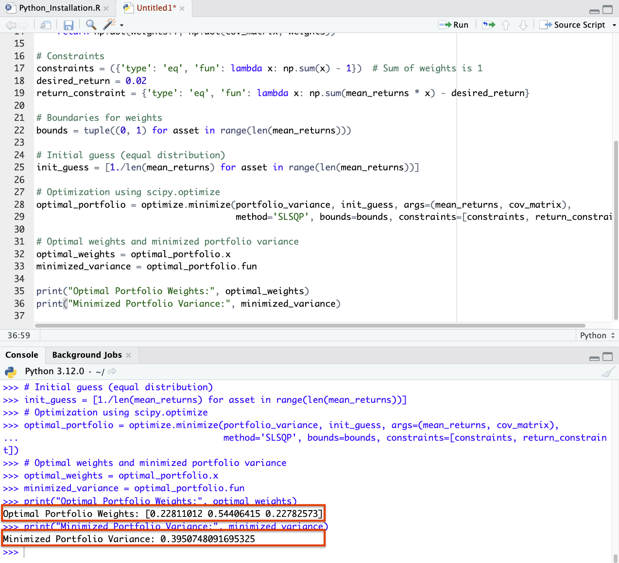
The 0.395 value represents the minimized risk of the portfolio under the constraint of achieving a certain level of return.
Now, in real-world scenarios, you would use actual historical return data or forward forecasts for the assets.
And the constraints (like desired return) would be based on the investor’s specific requirements and risk tolerance.
Also, other factors such as transaction costs, tax considerations, and liquidity constraints would also be involved in the optimization process.
But this is just an example so you get a feel for how the problem might be set up in Python.
FAQs – Conic Solvers in Financial Optimization Problems
What is global optimality?
Global optimality refers to the best possible solution across the entire range of possible solutions for an optimization problem.
In simpler terms, it’s like finding the lowest point in a landscape of hills and valleys – the point where you can’t go any lower, no matter where you start from.
What is a local minima?
A local minima is a solution that is the best in its immediate vicinity, but not necessarily the best overall.
Imagine being at the bottom of a small valley surrounded by higher ground – you’re at a low point, but there might be deeper valleys elsewhere.
Related