Volterra Processes in Finance & Trading

Volterra processes are used in various fields, including finance and economics.

They’re known for their versatility in modeling memory effects and non-Markovian dynamics that are often encountered in real-world systems.

Key Takeaways – Volterra Processes

• Memory Effect
  • Volterra processes incorporate history or “memory” of past values.
  • Allows traders to model asset prices with more realism.
  • Most appropriate in markets sensitive to past events/data (e.g., volatility tends to have a “memory”).
• Non-Markovian Dynamics
  • Unlike simpler models, they account for dependencies over time.
  • Important for accurately predicting the evolution of financial instruments under complex conditions.
• Flexibility in Modeling
  • Offers enhanced flexibility in capturing the volatility and correlation structures of financial markets.
  • “Memory” processes enable more sophisticated risk management strategies.
• Other Fields
  • Elsewhere, Volterra equations can model phenomena with hereditary/memory effects like populations dynamics, viscoelasticity, spread of disease.

Fundamentals of Volterra Processes

Volterra processes are defined through Volterra integral equations, where the future state of the system depends not just on its current state but also on its entire history.

Volteraa Processes Equations

A Volterra integral equation is an integral equation of the form:

y(t) = f(t) + ∫ K(t,s)y(s) ds

Where:

• y(t) – the unknown function to be solved for
• f(t) – the known inhomogeneous or free term
• K(t,s) – the kernel function
• s – the variable of integration

Key properties:

• The integration limit goes from 0 to t rather than -∞ to ∞ as in Fredholm equations. This makes Volterra equations effectively “one-sided.”
• Volterra equations exhibit a “memory” property – the value of y(t) depends on the history of y(s) for s ≤ t.
• The kernel K(t,s) represents the “memory” – it characterizes the influence of y(s) on y(t).

Volterra equations can be solved numerically by discretization or series approximation of the kernel.

This integral-based approach provides a robust framework for modeling systems where the past influences the future in a complex manner.

Unlike Markov processes, where the future is independent of the past given the present, Volterra processes retain a memory of past states.

This makes them suitable for more realistic models of financial markets where past events can have long-lasting effects.

Volatility as an Example of a Volterra Process

Volatility is probably the most common example of a Volterra process.

When volatility spikes in markets, it doesn’t go back to normal right away.

It generally takes a while.

Application of Volterra Processes in Financial Models

As mentioned, Volterra processes are increasingly used to model stochastic volatility, which is a key component in the pricing of financial derivatives.

The rough volatility model employs a Volterra process to capture the roughness observed in the volatility of financial markets.

This roughness, indicative of the irregular and jagged nature of market volatility, is well-represented by the fractional Brownian motion, a type of Volterra process.

By capturing these subtleties, Volterra processes offer a way to understand market dynamics and pricing complex financial instruments.

Volterra Processes & Risk Management

Risk management benefits significantly from the use of Volterra processes.

The ability of these processes to incorporate the history of a system allows risk managers to model and predict risk scenarios more accurately.

For instance, in credit risk modeling, the impact of past economic conditions on future defaults can be captured using Volterra processes.

This historical understanding can better inform risk models for the future.

Models Similar to Volterra Processes

Models similar to Volterra processes, which capture memory and non-Markovian dynamics in financial modeling, include:

Fractional Brownian Motion (FBM)

Extends the classical Brownian motion by incorporating a Hurst parameter, which allows for long-term memory effects in asset price movements.

Makes it suitable for markets with persistent trends or mean-reversion characteristics.

Autoregressive Conditional Heteroskedasticity (ARCH) and Generalized ARCH (GARCH) Models

Used for time series data, these models allow volatility to change over time based on past errors and variances.

This helps capture volatility clustering seen in financial markets.

Hawkes Processes

Capture self-exciting events, where the occurrence of an event increases the probability of future events.

Useful in modeling clusters of trades or financial contagion.

Stochastic Volatility Models

Such as the Heston model, which assumes that volatility itself follows a stochastic process, which allows for a more accurate description of market movements/properities.

These models share the ability to incorporate historical information and model financial markets forward.

Provides nuanced tools for risk management and option pricing.

Coding Example – Volterra Process

Implementing a Volterra process in the context of volatility modeling can be complex due to its integral and non-Markovian nature.

For financial applications, a common approach is to simulate paths using a discrete approximation.

Example #1

Below is a simplified Python code snippet that demonstrates how to simulate a rough volatility model (inspired by the Volterra process).

It focuses specifically on the rough volatility model framework, which is a practical application of Volterra processes in finance.

The rough volatility model, often exemplified by the rough Heston model, assumes that volatility dynamics are driven by a fractional Brownian motion, which is a type of Volterra process.

Due to the complexity of directly simulating fractional Brownian motion, we’ll use the Cholesky method for simplicity.

This acknowledges that there are more efficient methods for larger simulations or for a high degree of accuracy.

This example is highly simplified and intended for educational purposes. It illustrates the concept rather than providing a production-ready solution.

import numpy as np

def simulate_rough_volatility(T, N, H):
    """
    Simulate a rough volatility path using fractional Brownian motion via Cholesky decomposition.

    Parameters:
    - T: Total time horizon
    - N: Number of time steps
    - H: Hurst parameter, indicating memory and roughness (0 < H < 1)

    Returns:
    - A numpy array containing the simulated volatility path
    """
    # Time increment
    dt = T / N
    times = np.linspace(0, T, N+1)

    # Construct covariance matrix for fractional Brownian motion
    cov_matrix = np.zeros((N+1, N+1))
    for i in range(N+1):
        for j in range(i+1):
            cov_matrix[i,j] = 0.5 * (times[i]**(2*H) + times[j]**(2*H) - np.abs(times[i]-times[j])**(2*H))
            cov_matrix[j,i] = cov_matrix[i,j]

    # Cholesky decomposition to simulate correlated paths
     L = np.linalg.cholesky(cov_matrix)
     W = np.dot(L, np.random.normal(size=(N+1, 1))).flatten()

    # Assuming volatility is exp of fractional Brownian motion for positivity
    vol_path = np.exp(W)
    return vol_path

# Example parameters
T = 1 # 1 year
N = 250 # 250 time steps
H = 0.1 # Hurst parameter

vol_path = simulate_rough_volatility(T, N, H)

# Plot the simulated rough volatility path
import matplotlib.pyplot as plt

plt.plot(np.linspace(0, T, N+1), vol_path)
plt.title('Simulated Rough Volatility Path')
plt.xlabel('Time')
plt.ylabel('Volatility')
plt.show()

This code simulates a rough volatility path over a specified time horizon T, with N time steps, and a given Hurst parameter H.

The Hurst parameter controls the “roughness” of the volatility path, as we explained in more detail in our article on rough volatility.

Smaller values lead to rougher paths, which have been found to empirically match market data in some cases.

Example #2

This example uses basic Euler-Maruyama method (not the exact method for simulating fractional Brownian motion but can provide a rough approximation for educational purposes.)

import numpy as np

np.random.seed(15) 

def simulate_simple_rough_volatility(T, N, H):
    dt = T / N
    times = np.linspace(0, T, N+1)
    vol_path = np.zeros(N+1)
    vol_path[0] = 0.1 # Initial volatility value

    # Simplistically simulate changes in volatility
    for i in range(1, N+1):
        # Simplified placeholder for demonstration purposes
        dW = np.sqrt(dt) * np.random.randn()
        vol_path[i] = vol_path[i-1] + H * vol_path[i-1] * dW

    # Ensure all volatility values are positive
    vol_path = np.abs(vol_path)
    return vol_path, times

# Simulation
vol_path_simple, times_simple = simulate_simple_rough_volatility(T, N, H_adjusted)

plt.plot(times_simple, vol_path_simple)
plt.title('Simulated Rough Volatility Path (Simplified Model)')
plt.xlabel('Time')
plt.ylabel('Volatility')
plt.show()

Simulated Rough Volatility Path

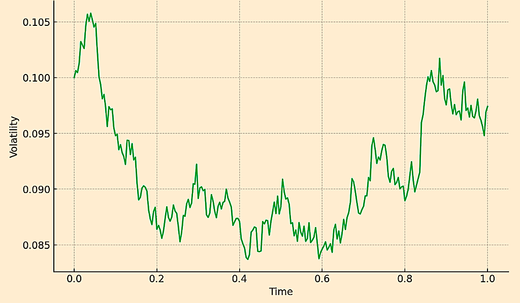
The graph above shows the simulated volatility path using a simplified rough volatility model.

This model doesn’t capture the full complexity of a true Volterra process or fractional Brownian motion, but provides a basic visualization of how volatility can evolve over time with roughness and memory effects.

Challenges & Computational Considerations

Volterra processes often leads to increased computational complexity, which is especially true for large datasets or complex models.

Efficient numerical methods and quality computing resources are typically required.

Conclusion

Volterra processes stand out modeling situations where past states significantly influence future dynamics and offer finer insights into complex, memory-influenced systems.

Their capacity to incorporate memory effects makes them valuable for applications like volatility and credit risk modeling.

Despite computational challenges, the depth and realism brought by Volterra processes into modeling efforts make them valuable in quantitative finance.