Rough Volatility & Bergomi Model (Applications & Coding Example)

Rough volatility models emerged from empirical observations that the volatility of financial markets does not behave smoothly.

Instead, it displays “roughness,” and needed better quantitative models to represent it accurately.

Key Takeaways – Rough Volatility & Bergomi Model

• Non-Smooth Volatility – Rough volatility models, including the Bergomi model, capture the observed rough, non-smooth nature of market volatility. Improves on assumptions of static volatility like many models.
• Improved Forecasting – These models provide more accurate short-term volatility forecasts. Important for options pricing and risk management.
• Complexity and Calibration – They are mathematically complex, requiring advanced techniques for calibration and implementation in trading strategies.

Understanding Rough Volatility

Traditional models, like the Black-Scholes model, assume that the volatility of asset prices is smooth and follows a certain predictable pattern.

In reality, financial markets often exhibit volatility that is far from smooth, with sudden spikes and drops.

This inconsistency led to the development of rough volatility models.

The term “rough” in rough volatility refers to the statistical property of the paths of volatility.

In mathematical terms, this roughness is often characterized by the Hurst parameter (H), where a parameter lower than 0.5 indicates roughness.

In rough volatility models, the Hurst parameter is usually estimated to be around 0.1.

Advantages of Rough Volatility Models

Rough volatility models provide several benefits, including:

Improved Calibration

These models can calibrate more accurately to market data.

This can help in the pricing of financial derivatives like options where volatility (implied volatility) is a key input.

Better Risk Management

By capturing the actual erratic behavior of market volatility, these models can help in more effective risk management strategies.

Forecasting Accuracy

They offer a more realistic framework for forecasting future market volatility by acknowledging the inherent roughness in market behavior.

The Bergomi Model: A Stochastic Volatility Model

The Bergomi model is a forward-looking stochastic volatility model used for pricing derivatives.

It’s most commonly used in markets where the volatility smile is prominent (which appears exactly as it seems).

It’s named after Lorenzo Bergomi, a quantitative researcher known for his contributions to stochastic volatility modeling.

Key Features of the Bergomi Model

Stochastic Volatility Dynamics

The model incorporates stochastic volatility.

This acknowledges that volatility isn’t constant but varies over time.

Volatility-of-Volatility

The Bergomi model allows for the volatility of volatility (“vol of vol”).

So it considers the variability in the volatility itself, which adds another layer of complexity and realism.

Leverage Effect Modeling

It accounts for the leverage effect, a phenomenon where asset prices and their volatility are often inversely related.

This is well-known in equities, for example.

Higher volatility is typically correlated with selling activity.

With something like oil, on the other hand, it can go both ways.

Oil can see volatility from selling off or can also see volatility from a geopolitical event (e.g., 1991 Gulf War, 2022 Russian invasion of Ukraine).

Forward Variance Curve

The model uses the concept of a forward variance curve, which represents the market’s expectation of future variance.

Markets are priced based on sets of discounted forward conditions, so this is important information.

Volatility traders and options traders are also aware of the concept of forward volatility.

Application of the Bergomi Model in Financial Markets

The Bergomi model is useful in equity and FX markets, where the volatility smile is a significant factor in pricing derivatives.

This leads to more accurate pricing and hedging of options and other financial derivatives.

What Are the Different Rough Volatility Models?

Rough volatility models have gained prominence in financial mathematics and quantitative finance for their capacity to capture the irregular and complex nature of market volatility.

Here are some of the notable rough volatility models:

1. Fractional Brownian Motion (FBM) Model

The FBM model extends the classical Brownian motion by incorporating memory effects and long-range dependence, characterized by the Hurst parameter H.

The key parameter, H, can take values in the range 0<H<1, where H<0.5 indicates roughness and long-term memory in volatility.

2. Rough Fractional Stochastic Volatility (RFSV) Model

Volatility Dynamics

This model captures the roughness by modeling the log volatility as a fractional Brownian motion with H<0.5.

Empirical Fit

RFSV models have been shown to fit the historical volatility of assets remarkably well.

This is also true in capturing the small-scale behaviors in financial time series.

3. Rough Bergomi Model

Enhancement of Bergomi Model

The Rough Bergomi model is an extension of the classical Bergomi model, incorporating roughness into the volatility dynamics.

Forward Variance Curve

It models the forward variance curve as being driven by a fractional Brownian motion.

This helps better capture the rough behavior of volatility.

4. Rough Volatility with Jumps

This model integrates jump components into the rough volatility framework to capture sudden and significant movements in asset prices.

It’s useful for modeling assets that exhibit jump risk or for scenarios like large market drops where traditional models fall short.

5. Multifactor Rough Volatility Models

These models consider multiple factors contributing to roughness.

This allows for a more comprehensive representation of volatility.

They accommodate various sources of market friction or multiple scales of market movements.

6. Hybrid Rough Volatility Models

Combination of Features

Hybrid models combine features of rough volatility models with other stochastic processes, like jump-diffusion models or mean-reverting processes.

Adaptability

They adapt to a wide range of market conditions and can capture both the continuous and discontinuous components of asset price dynamics.

Coding Example – Rough Volatility (Highly Simplified)

To model rough volatility, we can simulate a time series that captures the essence of rough volatility. 

Rough volatility models assume that volatility itself follows a stochastic process that isn’t necessarily smooth. 

A popular way to model this is by using a fractional Brownian motion, which is a generalization of the standard Brownian motion. 

But generating a fractional Brownian motion requires more complex methods.

For simplicity, let’s create a synthetic data series via numpy in Python that mimics rough volatility using a simpler method.

We’ll generate a time series where volatility changes over time in a non-smooth manner.

We’ll use Python to generate this data. Then plot the resulting graph of the price of the asset. 

This is just a simplified model to get your feet wet and doesn’t represent the complexity of actual rough volatility models used in financial mathematics.

import numpy as np
import matplotlib.pyplot as plt

# Set seed
np.random.seed(38)

# Gen synthetic price data
n = 252 # Trading days in a year
t = np.linspace(0, 1, n)
price_changes = np.random.normal(0, 1, n) # Daily returns (normally distributed)

# Create a simple rough volatility model
# Modulate the volatility by a random walk, which is non-smooth
volatility = np.abs(np.cumsum(np.random.normal(0, 0.02, n)))
price = 100 * np.exp(np.cumsum(volatility * price_changes)) # Simulate the price

# Plotting synthetic price data w/ rough volatility
plt.figure(figsize=(12, 6))
plt.plot(t, price)
plt.title("Synthetic Asset Price with Rough Volatility")
plt.xlabel("Time (Years)")
plt.ylabel("Price")
plt.grid(True)
plt.show()

And we get the following graph:

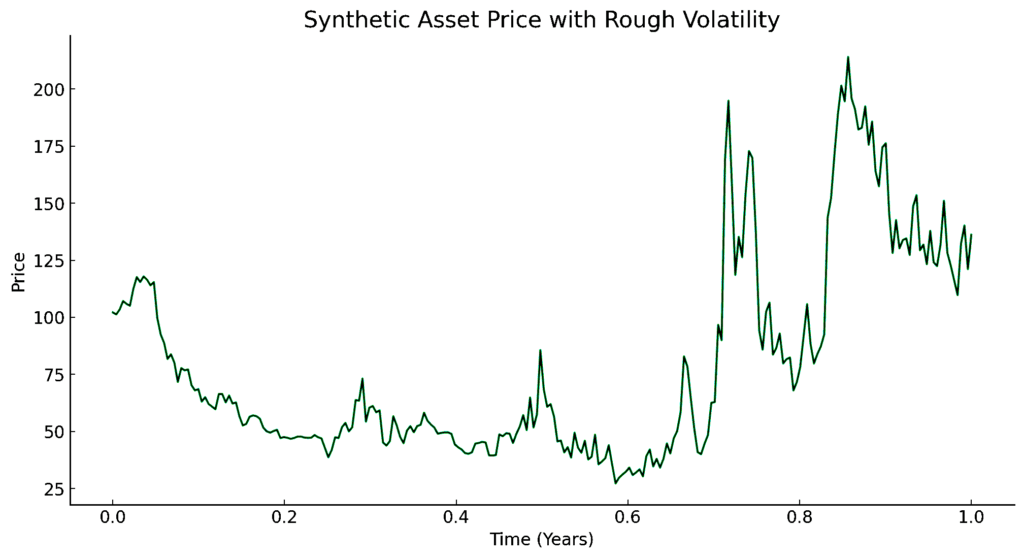
The graph represents a synthetic asset price series where volatility is modeled in a non-smooth manner, akin to a rough volatility model. 

The asset price evolves over time, influenced by daily returns and modulated by a random walk to simulate the rough nature of volatility.

Conclusion

Rough volatility and the Bergomi model address the limitations of earlier models that assumed too much smoothness in market volatility (such as the volatility assumptions underlying Black-Scholes).

These models help provide for more accurate pricing, risk management, and forecasting in financial markets.