Stochastic Discount Factor (SDF) Models

Stochastic Discount Factor (SDF) models are central to financial economics, as they provide a unified framework for understanding asset pricing.

These models, also known as pricing kernel models, are based on the concept that the price of an asset is the present value of its future payoffs, discounted by a stochastic process.

Key Takeaways – Stochastic Discount Factor (SDF) Models

• Pricing Mechanism
  • SDF models provide a unified framework to price assets by discounting their future payoffs.
  • Allows traders to evaluate investments’ present value based on expected returns and time value of money.
• Risk Adjustment
  • They incorporate risk adjustments directly into the discount factor.
  • Helps traders understand how risk levels affect asset prices and enabling more informed risk management decisions.
• Market Conditions Sensitivity
  • SDF models adapt to varying market/economic conditions (whatever parameters are coded into the model).
  • Shows how changes in economic factors impact asset valuations.
  • Facilitates dynamic/adaptive trading/investment strategies.

Here are the key concepts and types of SDF models:

Key Concepts

Stochastic Discount Factor (SDF)

A random variable that adjusts the future payoffs of an asset to its present value, accounting for time value of money and risk.

The SDF is stochastic.

This implies it can change unpredictably over time due to noise in how financial variables change.

No-Arbitrage Condition

SDF models are built on the no-arbitrage principle, stating that there should be no way to make a riskless profit from trading assets in efficient markets.

This principle ensures that asset prices are correctly priced relative to each other.

Risk-Neutral Pricing

Under certain conditions, SDF models can simplify to risk-neutral pricing, where the expected return on all assets is the risk-free rate.

In risk-neutral worlds, the SDF is related to the risk-free rate and doesn’t depend on investors’/traders’ risk preferences.

Market Completeness

A market is complete if the SDF is unique.

In complete markets, all risks can be perfectly hedged, and the SDF model provides a clear mechanism for asset pricing.

Incomplete markets, by contrast, may have multiple SDFs due to unhedgeable risks.

Equilibrium Models vs. Preference-Free Models

SDF models can be derived from equilibrium models, where the SDF is derived from:

• the optimization models of the market participant, or
• preference-free models –where the SDF is specified directly without reference to underlying economic agents‘ preferences

Types of Models

Consumption-Based Models

These models derive the SDF from the marginal utility of consumption.

The SDF is proportional to the ratio of marginal utilities at different times, which links asset prices to consumption patterns over time.

Factor Models

Factor models specify the SDF as a function of one or more risk factors.

The CAPM is a simple factor model with the market portfolio as the only factor.

Multifactor models include additional factors like size, value, and momentum.

Long-Run Risk Models

These models incorporate risks related to changes in the economic environment’s long-term outlook.

This affects consumption growth rates and investment/trading opportunities.

They often feature habit formation or external habit preferences.

Affine Models

In these models, the SDF is specified as an affine function of state variables.

Affine models are flexible and widely used in fixed income markets to model term structures of interest rates.

Disaster Risk Models

These models introduce rare but severe economic downturns (disasters) into the SDF framework.

They help explain asset price puzzles like the equity premium puzzle by accounting for the risk of catastrophic events.

Math Behind Stochastic Discount Factor Models

The stochastic discount factor (SDF) (aka the pricing kernel) is fundamental in asset pricing theory.

It allows you to price any asset by taking expectations.

SDF Formula

The basic formula is:

Price = E[SDF * Future Payoff]

Where:

• SDF = Stochastic discount factor
• E[] = Expectations operator
• Future Payoff = Random payoff of the asset in the future

For example, if we want to price a stock that pays a dividend Dt at time t, the formula is:

Stock Price = E[SDFt * Dt]

The SDF is a random variable that converts future payoffs into present values.

It reflects traders’/investors’ preferences and the market’s required compensation for risk.

Basic SDF Model

A basic SDF model is:

SDF = e^(-r*t) * (C/C0)^-γ

Where:

• e^(-r*t) = Time discounting factor
• C = Random consumption at time t
• C0 = Consumption today
• γ = Risk aversion coefficient

This shows the SDF declines exponentially with time and is lower in states where future consumption is high (investors need less compensation for risk).

More advanced SDF models incorporate multiple risk factors to explain asset returns.

But the basic math is to take expectations of the SDF multiplied by future payoffs to price assets.

The SDF is designed to capture all the market information about risk and return.

Coding Example – Stochastic Discount Factor Models

Here’s some basic Python code of how you might set up a simple stochastic discount factor model:

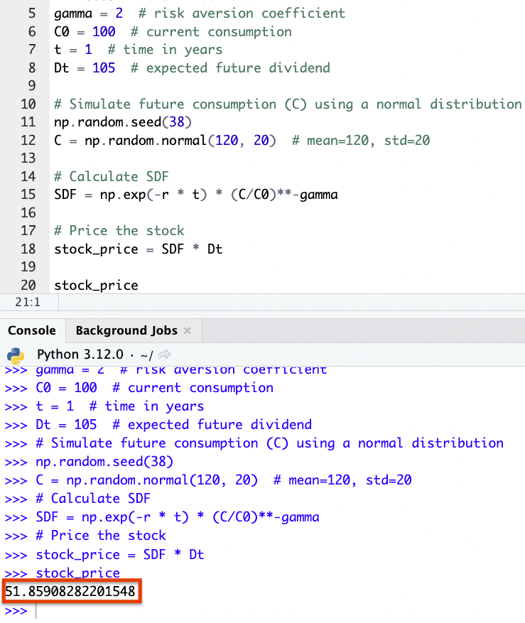
import numpy as np

# Define parameters
r = 0.03 # risk-free rate
gamma = 2 # risk aversion coefficient
C0 = 100 # current consumption
t = 1 # time in years
Dt = 105 # expected future dividend

# Simulate future consumption (C) using a normal distribution
np.random.seed(38) 
C = np.random.normal(120, 20) # mean=120, std=20

# Calculate SDF
SDF = np.exp(-r * t) * (C/C0)**-gamma

# Price the stock
stock_price = SDF * Dt

stock_price

Results

The calculated stock price (based on the specified stochastic discount factor model parameters and simulated future consumption) is approximately $51.86.

This example shows how the SDF model takes into account the time value of money, traders’/investors’ risk aversion, and the expected future payoff (in this case, a dividend) to determine the present value of an asset.

Conclusion

SDF models are used in financial economics to show how assets are priced and how markets respond to various risks and economic conditions.

They form the theoretical backbone for empirical asset pricing studies and financial market analysis.