Dynamic Stochastic General Equilibrium (DSGE) Models

Dynamic Stochastic General Equilibrium (DSGE) models are a class of macroeconomic models that are widely used in economic research and policy analysis.

Key Takeaways – Dynamic Stochastic General Equilibrium (DSGE) Models

• Macro-to-Micro Insights
  • DSGE models integrate macroeconomic theories with microeconomic foundations.
  • When done well, offer a comprehensive view of economic dynamics and policy impacts.
• Forward-Looking Analysis
  • They incorporate expectations and shocks.
  • Enables predictions about future economic conditions and their effects on markets.
• Complexity and Calibration Challenges
  • Despite their analytical value, DSGE models require precise calibration and face criticism for their assumptions and real-world applicability.

These models are characterized by the following features:

Dynamic

DSGE models examine how the economy evolves over time.

They do this by looking at how economic agents (like households, firms, and the government) make decisions across different periods, considering both current and future conditions.

Stochastic

These models incorporate stochastic (random) shocks.

These can be changes in technology, policy, preferences, or other external factors that affect the economy in unpredictable ways.

The stochastic nature of these models allows them to analyze how the economy responds to various unexpected events.

General Equilibrium

DSGE models consider the interactions of different sectors of the economy (such as consumers, producers, and the government) and how these interactions determine the allocation of resources across the economy in a way that supply equals demand in all markets simultaneously.

Microfoundations

They’re based on microeconomic principles.

This means that the behavior of the entire economy is derived from the optimizing behavior of individual agents.

For example, the model may assume that households maximize utility subject to budget constraints, and firms maximize profits.

Policy Analysis Tool

DSGE models are useful for conducting policy analysis.

They can simulate how an economy might respond to changes in policy, such as alterations in interest rates by central banks, fiscal policy changes by governments, and other regulatory interventions.

Calibration & Estimation

To make these models useful for real-world economies, they need to be calibrated or estimated using actual economic data.

This process involves setting the values of various parameters in the model (like how sensitive consumers are to changes in interest rates) so that the model’s behavior mirrors real-world data as closely as possible.

DSGE Models – Strengths & Weaknesses

DSGE models have both strengths and criticisms.

Their main strength lies in their theoretical foundations and their ability to simulate the effects of different policies before they’re implemented.

But they’re often criticized for their reliance on certain controversial assumptions (like rational expectations and representative agents) and for sometimes failing to predict or account for major economic events, like the financial crisis of 2007-2008, due to missing (or inappropriately underweighted or overweighted) variables.

DSGE Models for Markets & Trading

In the context of financial markets, DSGE models can be used to understand macroeconomic dynamics and their potential impacts on asset prices, market strategies, and risk assessments.

Nonetheless, the complexity and assumptions underlying DSGE models mean that they should be used with caution and in conjunction with other types of analysis.

Python DSGE Model

Creating a basic Dynamic Stochastic General Equilibrium (DSGE) model in Python with synthetic data involves several steps.

We’ll use a basic New Keynesian DSGE model, which includes elements such as a representative household, a production function, and a monetary policy rule.

The model will be highly simplified and abstracted for illustration purposes.

It will include the following components:

• Households – They maximize utility over consumption and labor supply.
• Firms – They produce goods/services using labor and technology.
• Monetary Authority – Sets the interest rate according to a Taylor rule.

For the sake of simplicity, we’ll omit many real-world complexities like capital accumulation, government sector, and investment dynamics.

We’ll also assume that all parameters are known and fixed.

This code snippet sets up a basic DSGE model with some key economic variables and relationships.

It then simulates the model over 100 periods with random technology shocks and plots the key variables’ trajectories.

Note that this is a highly stylized model, and real-world applications would require more sophisticated setups and data considerations.

Also, the process of solving a DSGE model can be more complex. It often requires numerical methods such as the perturbation method or value function iteration.

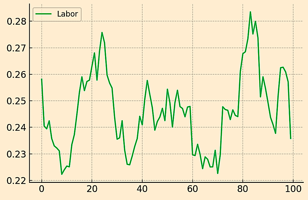
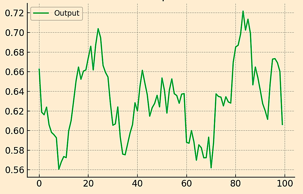
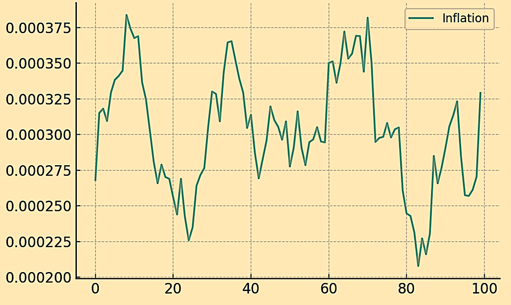
From the code we generate the following plots:

Labor

Output

Output effectively matches labor, given labor is typically taken to be the same as output.

Inflation

The code:

import numpy as np
import matplotlib.pyplot as plt
from scipy.optimize import fsolve

# Parameters & functions
beta = 0.99 # Discount factor
alpha = 0.33 # Labor share
phi_y = 0.125 # Taylor rule parameter (output)
phi_pi = 1.5 # Taylor rule parameter (inflation)
sigma = 1.0 # Elasticity of substitution in consumption
epsilon = 6.0 # Elasticity of substitution in production
rho = 0.9 # Autocorrelation of technology shock
sigma_z = 0.02 # Standard deviation of technology shock

# Steady state values
ss_y = 1.0 # Output
ss_c = 0.7 # Consumption
ss_l = 0.3 # Labor
ss_pi = 0.02 # Inflation
ss_r = 1.01 # Nominal interest rate
ss_z = 1.0 # Technology shock

# Equilibrium conditions
def corrected_equilibrium(vars, z):
    c, l, pi, y, r = vars
    y_e = production(l, z)
    r_e = taylor_rule(pi, y)
    euler_eq = beta * (c / ss_c)**(-sigma) * (1 + pi) - (1 + r_e)
    labor_supply_eq = (c / ss_c)**(-sigma) - alpha * y_e / l
    production_eq = y - y_e
    inflation_eq = epsilon / (epsilon - 1) - c / ss_c
    interest_rate_eq = r - r_e # Corrected to include an equation for the interest rate
    return [euler_eq, labor_supply_eq, production_eq, inflation_eq, interest_rate_eq]

# Simulate the model using the corrected equilibrium function
z_series_initial = np.random.normal(0, sigma_z, T+1) # Generating T+1 to ensure the AR process can be applied
z_series = np.empty(T)
z_series[0] = z_series_initial[0]
for t in range(1, T):
    z_series[t] = rho * z_series[t-1] + z_series_initial[t]

# Store results in arrays
c_series = np.zeros(T)
l_series = np.zeros(T)
pi_series = np.zeros(T)
y_series = np.zeros(T)
r_series = np.zeros(T)

for t in range(T):
    z = ss_z * np.exp(z_series[t]) # Convert to level
    vars_initial = [ss_c, ss_l, ss_pi, ss_y, ss_r] # Initial guesses for the fsolve
    c, l, pi, y, r = fsolve(corrected_equilibrium, vars_initial, args=(z,))
    c_series[t], l_series[t], pi_series[t], y_series[t], r_series[t] = c, l, pi, y, r

# Plotting the corrected results
plt.figure(figsize=(12, 8))
plt.subplot(221)
plt.plot(c_series, label='Consumption')
plt.title('Consumption')
plt.legend()
plt.subplot(222)
plt.plot(l_series, label='Labor')
plt.title('Labor')
plt.legend()
plt.subplot(223)
plt.plot(pi_series, label='Inflation')
plt.title('Inflation')
plt.legend()
plt.subplot(224)
plt.plot(y_series, label='Output')
plt.title('Output')
plt.legend()
plt.tight_layout()
plt.show()