Agent-Based Modeling (ABM) in Finance

Agent-Based Modeling (ABM) is a very important aspect of financial market analysis and prediction, but is one of the least talked about.

It operates under a different paradigm compared to traditional economic and financial models, which often rely on equilibrium theories (e.g., value investing, discounted cash flow) and aggregate market behaviors.

In ABM, the market is viewed as a complex system composed of various agents (individuals or entities) with distinct behaviors and interactions.

In reality, ABM is about:

• identifying the buyers and sellers
• estimating how much they’re likely to impact supply and demand
• how this picture changes based on variables that impact their actions (e.g., changes in discounted growth, discounted inflation, discount rates, risk premiums, regulation, and so on)

Under the ABM framework, it all comes down to who’s going to buy and who’s going to sell and for what reasons.

That’s the whole idea.

Most market commentary skips past it.

Analysts talk about “the market” as if it were one thing.

They speak of valuations as if prices were set by a committee of rational beings looking at fundamentals. If something if “off” they can’t figure out why.

They forecast based on equilibrium models that assume away the very thing that actually moves prices – which is the messy, mismatched, motivated behavior of real participants doing real things with real money.

ABM strips away the abstraction and asks the only question that matters at the transaction level. Who is buying? Who is selling? Why? And how big are they?

Think of the economy at a basic mechanistic level. Spending comes in the form of either money or credit. Every transaction has a buyer on one side and a seller on the other. Most of what people think is money is really credit, and credit does appear out of thin air during good times and then disappear at bad times.

None of this happens in the aggregate. It happens at the level of individual decisions made by individual entities for individual reasons. ABM is the analytical framework that takes those individual decisions and brings them back up to aggregate market movements.

Key Takeaways – Agent-Based Modeling (ABM)

• Individual Agent Focus – ABM in finance emphasizes the unique behaviors and interactions of individual market participants, rather than relying on aggregate market assumptions.
  • Who are the buyers and sellers? How big are they? What are they motivated to do?
  • Enables a more nuanced understanding of market dynamics.
  • Instead of considering “the market” to be a monolithic entity or basing decisions on notional equilibrium values, it’s about who’s buying and who’s selling and for what reasons.
• Data Intensity – ABM requires extensive data on “agent” behaviors.
• Example – We do a Python example of agent-based modeling later on in this article.

Why Equilibrium Models Fall Short

The classical equilibrium framework assumes that markets clear at prices reflecting some “true” fundamental value, that participants are rational, and that information is processed uniformly.

But none of these assumptions holds in any market you’ll observe.

Unfortunately for the value crowd, markets don’t clear at fundamental values.

They clear at the price where the marginal buyer meets the marginal seller, and the marginal buyer is often a forced buyer (e.g., a pension fund mandated to hold duration), and the marginal seller is often a forced seller transacting (e.g., a government selling debt to fund their deficits, a sovereign wealth fund selling per their mandates). Neither of them necessarily cares about discounted cash flows in that moment. They care about what their mandates and constraints require them to do.

Said differently: prices are set by flows, and flows are set by motivations and constraints, not by fundamentals. The extent to which they influence prices depends on their relative sizes in the individual markets.

This is why two analysts looking at the same earnings report can produce wildly different price targets and both be wrong. They are forecasting fundamentals when they doesn’t have much to do prices in the moment – or even over a handful of years.

That’s why more sophisticated macro- and quant-oriented traders model participants. ABM forces you to ask: given what is happening, who is now compelled to act, and in what direction?

Key Components of Agent-Based Modeling in Financial Markets

Identification of Agents

This involves categorizing market participants as buyers or sellers.

Each agent is characterized by unique objectives, constraints, and decision-making processes.

In financial markets, these agents can range from individual investors and institutional traders to automated trading algorithms.

A practical taxonomy looks something like this:

On the institutional side: pension funds, insurance companies, sovereign wealth funds, central banks, commercial banks, asset managers, hedge funds, market makers, and dealer balance sheets. (Related: 17+ Institutional Participants to Know in Markets)

On the retail side: individual investors with brokerage accounts, robo-advised allocations, and 401(k) flows.

On the algorithmic side: high-frequency traders, statistical arbitrage funds, trend followers like CTAs, and risk-parity portfolios.

Each of these has a different mandate, a different time horizon, a different constraint set, and a different set of triggers that move it from neutral on existing positions to active in markets.

The first job of the agent-based modeler is to know who is in the market.

Agent Characteristics

Understanding the size and influence of each agent is key.

In financial markets, this might refer to the capitalization or trading volume controlled by an agent.

Larger agents (like institutional investors) can have a material effect on markets through their buying and selling activity.

Size has an influence in a non-linear way.

A pension fund running $500 billion doesn’t just have a hundred times the impact of a $5 billion family office. Its trades are slower, its rebalancing is calendar-driven, and its positioning is constrained by liability matching rules that don’t apply to anyone else.

A central bank running open market operations is a different category of agent altogether. When the Federal Reserve buys $80 billion of Treasuries a month, the question of who is on the other side of that trade reshapes the entire term structure. Size isn’t only a multiplier on impact, but a determinant of behavior.

Agent Motivations and Behaviors

This is arguably the most complex aspect.

Agents’ decisions in financial markets are influenced by various factors, including, but not limited to:

Economic Indicators

Changes in macroeconomic factors like growth and inflation, often heavily viewed in the form of future expectations (discounted growth and inflation).

Discount rates and risk premiums also influence decisions.

Regulatory Environment

Changes in financial regulations can alter the “rules” of how participants engage in markets and what markets they participate in.

Information Asymmetry and Market Signals

How agents interpret and react to market information.

Technological Changes

The impact of new technologies on market operations and strategies.

So, motivations aren’t uniform.

A pension fund and a hedge fund can be looking at the same 10-year Treasury yield and reach opposite conclusions about whether to buy.

The pension fund sees a yield that helps it match its long-dated liabilities and reduces its funding gap.

The hedge fund sees a yield that’s too low relative to its inflation forecast and shorts the bond (or sells what it has). Both decisions are rational in their own context. The price you observe is what falls out of all those rational decisions colliding.

So, the market isn’t making one decision. It’s the residue of many decisions made for many reasons.

How Agent-Based Modeling Predicts Market Movements

Emergent Phenomena

Unlike traditional models, ABM can capture emergent phenomena.

These are outcomes that arise from the interactions of individual agents – but are not predictable from the characteristics of the agents themselves.

This includes market trends and bubbles.

A bubble is a classic emergent outcome. No single participant decides to create a bubble.

It emerges from the interaction of:

• momentum traders chasing prices
• leveraged buyers stretching to participate
• retail investors piling in late, and
• risk managers raising position limits as volatility falls and Sharpe ratios rise

Each individual decision looks defensible in isolation. The aggregate is unstable. ABM captures this. Equilibrium models can’t.

Scenario Analysis

Simulating various scenarios considering different actions and reactions of agents can help in understanding potential future market movements.

The power here is being able to ask conditional questions.

What happens if the Fed unexpectedly cuts rates by 50 basis points? In a traditional model, you adjust a few parameters and read off a new equilibrium.

In ABM, you ask which agents become more or less constrained, which agents have new opportunities, which agents are forced to rebalance, and what the second-order/nth-order effects look like as their trades hit the order book.

Non-linear Dynamics

Financial markets are inherently non-linear. Small changes can have disproportionately large effects.

ABM is well-suited to model these dynamics due to its focus on individual interactions.

Non-linearity comes from thresholds. A bank that has been holding a security has no reason to sell at any price above its accounting cost. The moment the price drops below that threshold, the bank is forced to mark down, recognize losses, and potentially sell.

The same one-cent move in price has zero effect on day one but can have a big effect on day two. Aggregate models will smear this out. But a well-built ABM can capture it.

Feedback Loops

ABM can incorporate feedback loops where the actions of agents influence the market, which in turn influences the agents. This leads to complex dynamic patterns.

The classic feedback loop in financial markets is the wealth effect, but it runs both directions.

Rising asset prices make holders feel richer, which encourages more lending and more spending, which raises asset prices further.

Falling asset prices do the opposite. As wealth falls first and incomes fall later, creditworthiness worsens, which constricts lending activity, which hurts spending and lowers investment rates while also making it less appealing to borrow to buy financial assets. This in turn worsens the fundamentals of the asset, leading people to sell and driving down prices further. This has an accelerating downward impact on asset prices, income, and wealth.

These dynamics are core features of financial markets.

Challenges

Model Complexity

ABMs can become exceedingly complex and require substantial computational resources, especially as the number of agents and the complexity of their interactions increase.

There is a real engineering tradeoff here. A model with 50 agent types each with 20 parameters is already running in a 1,000-dimensional parameter space. Calibrating such a model is hard. Validating it is harder.

The temptation is to add detail because every additional behavioral rule looks reasonable in isolation. Keep the model simple enough to actually understand. A simple model that captures the dominant dynamic beats a complex model that captures everything but cannot be reasoned about.

Data Requirements

Accurate modeling requires detailed data about agents and their behaviors. Naturally, this can be difficult to obtain.

Position data for institutional investors is partially available through 13F filings, COT (Commitment of Traders) reports, central bank balance sheet disclosures, and TIC (Treasury International Capital) data. Flow data is available from fund-level disclosures and ETF creation/redemption activity.

Behavioral data, the rules each agent follows in response to what happens (i.e., variables of importance), is much harder. Pensions have certain allocations they follow as one example (many of which are published). It has to be inferred from public mandates, regulatory filings, and observed historical behavior.

Building this dataset is most of the work in any serious ABM project.

Parameter Sensitivity

ABMs can be sensitive to initial conditions and parameter choices. This makes them challenging to calibrate and validate against real-world data.

Two ABMs with slightly different starting positions can produce dramatically different paths.

Best practices generally involve running thousands of simulations with varied initial conditions and parameter draws, and look at the distribution of outcomes rather than any single trajectory. The idea is to understand which scenarios are likely, which are tail events, and understand what you might be missing.

Agent-Based Modeling Example

To illustrate Agent-Based Modeling (ABM) in the context of the US Treasury market, let’s consider a simplified scenario with key agents categorized as buyers and sellers, along with their motivations.

Agents in the US Treasury Market

Sellers:

• US Government – Issues Treasury bonds primarily to finance government spending.
• Federal Reserve – May sell (sometimes buy) Treasuries as part of its monetary policy operations.
• Individual Entities – Include private traders/investors, who may sell Treasuries for portfolio rebalancing or liquidity needs.

Buyers:

• Pension Funds – Buy Treasuries for long-term income stability and to match their long-dated liabilities.
• Commercial Banks – Purchase Treasuries as High-Quality Liquid Assets (HQLA) for regulatory liquidity requirements and for income.
• Retail Investors – Attracted to Treasuries for their safety and income.
• Hedge Funds – May buy Treasuries for strategic trading, hedging, or arbitrage opportunities.
• Central Banks and Reserve Managers – Buy US Treasuries to manage foreign exchange reserves, often seeking safety and liquidity.

The main takeaway is the Treasury market isn’t one thing, but the collision of these specific participants doing specific things for specific reasons.

Modeling their Motivations and Interactions

Interest Rate Movements

A rise in interest rates might lead pension funds to increase their Treasury holdings for better yields.

On the other hand, hedge funds might short them.

Economic Policy Changes

If the Federal Reserve signals tightening monetary policy, commercial banks might adjust their Treasury holdings – e.g., buying shorter-term bonds to lower duration risk.

Market Sentiments

In times of higher market volatility, traders might increase their Treasury holdings, looking for safety over higher returns.

Regulatory Changes

If regulatory requirements for HQLA are increased, commercial banks may respond by boosting their Treasury holdings.

Global Economic Factors

International central banks might adjust their Treasury investments in response to global growth and inflation conditions, which affect supply and demand dynamics. Hedging costs are a factor of how economic these trades are.

In bond markets, domestic buyers care about real returns (nominal return minus inflation, focusing on buying power). International buyers also have to factor in currency movements.

Simulating Market Dynamics

Examples:

Scenario 1: Economic Downturn

In this scenario, retail and institutional investors might flock to Treasuries as a safe haven, driving up prices.

The Federal Reserve might add to this by buying Treasuries to inject liquidity into the market.

Runs from risky assets to less risky assets pick up, which contributes to a broadening of the contraction. Liquidity becomes a major concern.

Government bonds become the safe haven. The flow into Treasuries is not because anyone calculates a new fair value. It’s because risk managers across thousands of institutions hit the same de-risking triggers at roughly the same time, and the only asset that satisfies all their constraints simultaneously is the front end of the Treasury curve.

Scenario 2: Rising Interest Rates

This could lead to a sell-off in Treasuries – particularly by short-term investors and hedge funds.

Long-term holders like pension funds might be less reactive, considering their long-term income goals.

This is a useful place to see how heterogeneity matters. The same rate move that causes a leveraged macro fund to puke its long bond position causes a pension fund to add.

Why?

Because the pension fund’s liabilities are also being repriced by the same move, and the higher discount rate reduces the present value of those liabilities.

Net of liabilities, the pension is now under-hedged on duration and needs to buy. Same data, opposite trade. Equilibrium models will not factor this in, but ABM can.

Scenario 3: Regulatory Shift

An increase in HQLA requirements could see a surge in demand from commercial banks, which impacts Treasury yields and market liquidity.

Regulatory shifts are some of the cleanest ABM case studies because the affected agents are easy to identify and their constraints are explicit.

When Basel III phased in liquidity coverage ratio requirements, it created a structural buyer of high-grade sovereign debt that didn’t exist before.

The flows showed up in the term structure well before any fundamental “fair value” reason emerged.

Coding Example – Agent-Based Modeling

Let’s do an example.
In this simulation:

• Each agent has unique sensitivities to the economic factors and makes buy or sell decisions based on a weighted sum of these factors.
• Daily fluctuations in the economic factors are introduced, mimicking real-world variability.
• The collective decisions of all agents result in a net position each day, which influences the Treasury price.

The economic factors are discounted growth, discounted inflation, discount rates, and risk premiums. (Related: 4 Variables that Determine Financial Asset Pricing)

The Treasury price fluctuates in response to the aggregated decisions of the agents.

This demonstrates how individual behaviors and market conditions can impact financial instruments in a simplified ABM framework.

This Python model provides a basic understanding of how ABM can be used to study complex financial markets (albeit in a highly stylized manner).

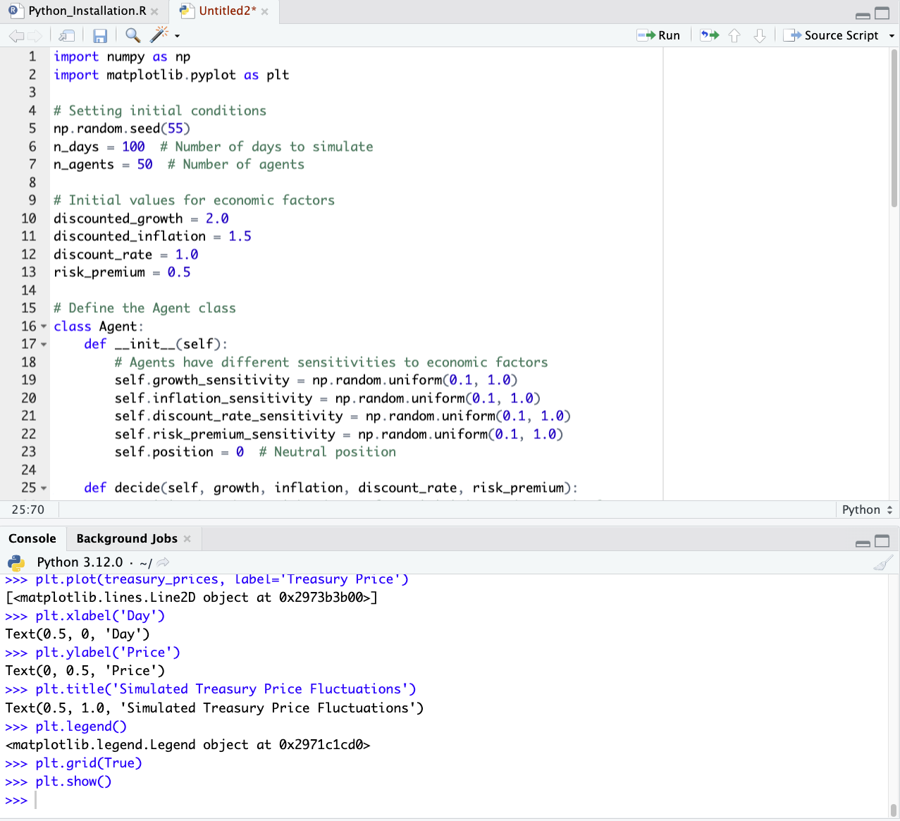
Agent-Based Modeling in Python

import numpy as np
import matplotlib.pyplot as plt
# Setting initial conditions
np.random.seed(55)
n_days = 100 # Number of days to simulate
n_agents = 50 # Number of agents
# Initial values for economic factors
discounted_growth = 2.0
discounted_inflation = 1.5
discount_rate = 1.0
risk_premium = 0.5
# Define the Agent class
class Agent:
def __init__(self):
# Agents have different sensitivities to economic factors
self.growth_sensitivity = np.random.uniform(0.1, 1.0)
self.inflation_sensitivity = np.random.uniform(0.1, 1.0)
self.discount_rate_sensitivity = np.random.uniform(0.1, 1.0)
self.risk_premium_sensitivity = np.random.uniform(0.1, 1.0)
self.position = 0 # Neutral position
def decide(self, growth, inflation, discount_rate, risk_premium):
# Decision based on weighted sum of sensitivities and economic factors
decision_score = (self.growth_sensitivity * growth 
- self.inflation_sensitivity * inflation 
- self.discount_rate_sensitivity * discount_rate 
+ self.risk_premium_sensitivity * risk_premium)
if decision_score > 0:
self.position += 1 # Buy or increase holding
elif decision_score < 0:
self.position -= 1 # Sell or decrease holding
# Initialize agents
agents = [Agent() for _ in range(n_agents)]
# Lists to store simulation results
treasury_prices = []
# Simulation loop
for day in range(n_days):
# Random fluctuation in economic factors
discounted_growth += np.random.uniform(-0.05, 0.05)
discounted_inflation += np.random.uniform(-0.05, 0.05)
discount_rate += np.random.uniform(-0.02, 0.02)
risk_premium += np.random.uniform(-0.02, 0.02)
# Agents make decisions
for agent in agents:
agent.decide(discounted_growth, discounted_inflation, discount_rate, risk_premium)
# Calculate net position of all agents
net_position = sum(agent.position for agent in agents)
# Adjust Treasury price based on net position
# Base price is 100, and each net position unit changes the price by 0.1
treasury_price = 100 + 0.1 * net_position
treasury_prices.append(treasury_price)
# Plotting the results
plt.figure(figsize=(12, 6))
plt.plot(treasury_prices, label='Treasury Price')
plt.xlabel('Day')
plt.ylabel('Price')
plt.title('Simulated Treasury Price Fluctuations')
plt.legend()
plt.grid(True)
plt.show()

If using this code, please be sure to indent as needed, as this is necessary in Python syntax:

At the end, we get a plot of the simulation:

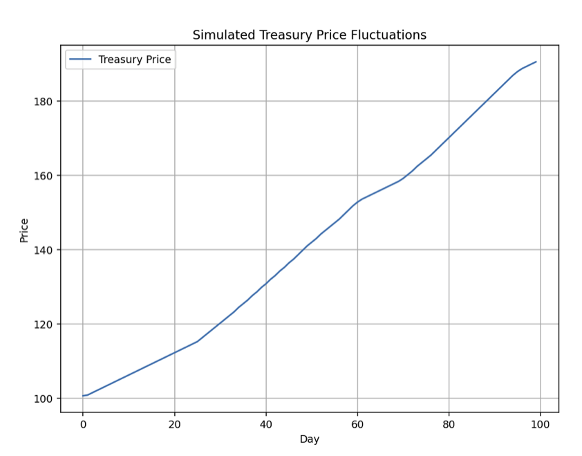
The plot above illustrates the simulated fluctuations in the Treasury price over a period of 100 days, based on the decisions of individual agents in response to changes in discounted growth, inflation, discount rates, and risk premiums.

Reading the Output Like a Practitioner

What the chart shows is a path. One realization out of an infinite number of possible realizations consistent with the agent rules and the input dynamics. If you re-ran the same code with a different random seed, you would get a different chart. That’s the right way to think about ABM output. It is a sample from a distribution of possible futures, not a prediction of the actual future.

For example:

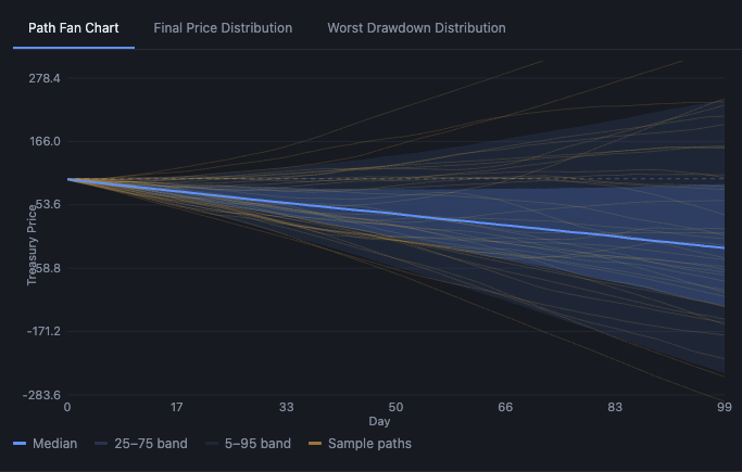
The useful question to ask of an ABM output is not “where will the price be in 100 days?” The useful question is: across thousands of simulated paths, what is the distribution of outcomes, and what conditions cause the worst paths? That distributional view is what informs position sizing and hedging decisions. A point forecast is ultimately nonsense.

Extending the Model: What Real Practitioners Do Next

The toy model above has 50 identical-architecture agents with random sensitivities. That is not how real markets work. Real markets have a small number of larger agents and a large number of smaller ones. The large agents have very specific, often public, mandates. The small agents are more random but matter less individually.

A more realistic ABM would do at least the following.

Distinguish Agent Types

First, distinguish agent types rather than just sampling sensitivities.
A pension fund agent should have a buy rule triggered by the funded ratio dropping below a threshold. A hedge fund agent might have a leverage constraint. A central bank agent should have a balance sheet target. These are explicit policies.

Model the Order Books

Second, model the order book, not just the net position. Markets clear because someone posts a bid and someone hits an offer. The microstructure of who provides liquidity and who takes it is itself a determinant of price impact. A net buying flow of $10 billion in a deep market moves prices very little. The same flow in a thin market or during a stress period can move prices several percent.

Map Price to Behavior

Third, include the feedback from price to behavior. A 5% drop in Treasury prices triggers VaR-based de-risking at some funds and triggers buying at others (the pension example above).
The fact that the price move itself changes who is buying and selling is the heart of why markets are non-linear. The model needs to capture this.

Policy Reaction Function

Fourth, incorporate the policy reaction function. The Federal Reserve does not act mechanically based on a Taylor rule. It reacts to financial conditions, to political pressure, to its own forecasts of growth and inflation, and to the behavior of other agents. Modeling the central bank as just another agent, with its own rule set and triggers, is essential when the model is being used to study sovereign debt markets.

Map How the Agent Population Changes Over Time

And fifth, allow the agent population itself to change. Bull markets attract new entrants. Bear markets remove them. The composition of the market in 2007 was different from the composition in 2009, which was different from 2021.

A static agent population captures dynamics within a narrow point in time. A model that allows agents to enter and exit, become bigger and smaller, evolve mandates, etc., is a step in the right direction.

What ABM Tells the Trader

Before taking a view on a market, ask:

• Who has been the dominant buyer?
• What is their motivation?
• What conditions would change their behavior?
• Who is on the other side, and at what point do they step up?
• When the conditions change, what does the order book look like?

Markets that look stable on the surface can be unstable in their agent composition. A bond market held by leveraged carry traders looks the same as a bond market held by long-term reserve managers, until something forces the leveraged traders to delever. Then they look very different. The price discontinuity that follows isn’t random. It is the predictable consequence of an agent-composition shift that any ABM-aware analyst could have flagged.

Said differently: the right question is rarely “is this asset cheap?” The right question is “who owns it, why do they own it, and what would make them stop owning it?”

That’s the main value of the framework.

Conclusion

Equilibrium models are useful for thinking about long-run averages. Unfortunately, they are nearly useless for understanding what happens between now and the long run, which is where market participants actually have to operate.

ABM fills that gap. It treats the market as what it actually is: a set of motivated, heterogeneous, constrained participants whose interactions produce the prices we observe.

It refuses the convenient fiction that “the market” is a single thing with a single view. It demands specificity.

That specificity is hard. It requires data, computation, and judgment.

But the alternative is to keep using models that smooth over the very features of markets that drive returns, and to be repeatedly surprised by outcomes that any practitioner who actually knew the participants could have anticipated.

Consider every market you trade in “agent” terms. Who is buying. Who is selling. Why. How big. What changes their mind. Then, if you’re interested, build the model.