Variance Gamma Process

The Variance Gamma (VG) process is a mathematical model used in financial markets for option pricing and to capture the dynamics of asset returns.

It’s noted for its ability to model the skewness and leptokurtosis (fat tails) observed in the distribution of returns – characteristics often inadequately captured by the simpler Black-Scholes model, which assumes lognormal distribution and constant volatility.

The VG process introduces “jumps” in asset prices and stochastic volatility, which offers a more accurate representation of market behaviors.

Key Takeaways – Variance Gamma Process

• Captures Extreme Moves
  • The Variance Gamma process models market dynamics, including rare but impactful extreme movements.
  • Important for traders managing tail risks.
• Incorporates Skewness and Leptokurtosis
  • VG addresses the limitations of traditional models by capturing the actual skewed and fat-tailed distribution of returns.
  • Offers better pricing and risk assessment.
• Enhances Option Pricing
  • It provides a more realistic framework for pricing options, especially for assets with observable jumps and varying volatility.

Here are the key concepts and applications related to the VG process:

Key Concepts of Variance Gamma Process

Stochastic Volatility & Jumps

Unlike models that assume constant volatility, the VG process incorporates both stochastic volatility and jumps in asset prices.

Reflects more accurately the empirical observations of financial markets.

Gamma Process

The VG model is constructed by subordinating a Brownian motion to a gamma process.

The gamma process introduces the “time change” element, where the amount of variance (volatility) in the Brownian motion is itself random, modeled by a gamma distribution.

This results in a model that can produce returns with skewness and kurtosis.

Leptokurtosis

The VG process is capable of capturing leptokurtosis, which is the presence of fat tails in the distribution of returns.

This means it can more accurately model the probability of extreme market movements.

Skewness

It also allows for the modeling of skewness in the distribution of returns, where the distribution can lean toward either more positive or negative returns, a common observation in real-world financial markets.

Math Behind the Variance Gamma Process

Here’s an overview of the math behind the Variance Gamma process:

Key Idea

Model stock returns using a drifted Brownian motion subordinated by a Gamma process.

• Xt = θGt + σW(Gt)

Where:

• Xt is the VG process
• θ is the drift rate
• σ is the volatility
• W(t) is a Brownian motion
• Gt is a Gamma process with mean rate 1/ν

Properties

• Leads to heavier tails than Gaussian
• Allows flexible asymmetry and kurtosis
• Has independent, stationary increments
• Analytic characteristic function

The math uses:

• Time changes and subordination of processes
• Gamma process properties
• Characteristic functions and Levy processes

Overall, VG processes provide a tractable way to introduce non-Gaussian behavior into asset return models using probabilistic subordination and time change techniques.

The math enables fitting financial time series with additional flexibility.

Applications of Variance Gamma Process

Option Pricing

The VG process is widely used for pricing European and exotic options, where traditional models like Black-Scholes might fail to capture market nuances.

It provides more accurate pricing by accounting for the observed market skewness and kurtosis.

Risk Management

By more accurately modeling the tails of the distribution of returns, the VG process helps in better quantifying and managing the risk of extreme market movements, which is important for portfolio management and financial planning.

Market Analysis

Traders and analysts use VG models to assess the probability of large jumps in asset prices.

This can be critical for short-term trading strategies and for hedging against market downturns.

Fixed Income Securities

VG processes can also be applied in the fixed income market to price bonds and other interest rate derivatives, where the assumptions of normality and constant volatility generally don’t hold.

Volatility Trading

The model’s ability to incorporate stochastic volatility makes it useful for trading volatility as an asset class, such as through VIX options, variance swaps, and other volatility products.

Coding Example – Variance Gamma Process

Let’s do a coding example of a Variance Gamma process.

import numpy as np
import matplotlib.pyplot as plt

# Parameters for the Variance Gamma process
T = 1 # Time horizon
sigma = 0.12 # Volatility parameter for the Brownian motion part
nu = 0.1 # Rate of drift of the Variance Gamma process
theta = -0.14 # Drift of the Brownian motion part
gamma = 0.2 # Parameter to control the variance of the gamma process

# Time parameters for simulation
N = 1000 # Number of steps
dt = T/N # Time step

# Sim the Variance Gamma process
# Step 1: Simulate the Gamma process
t = np.arange(0, T, dt)
G = np.random.gamma(shape=dt/gamma, scale=gamma, size=N)

# Step 2: Simulate the Brownian motion part
W = np.random.normal(loc=0, scale=np.sqrt(dt), size=N)
X = theta*G + sigma*np.sqrt(G)*W + nu*G

# Compute cumulative sum to get the process values
S = np.cumsum(X)

# Plot the Variance Gamma process
plt.figure(figsize=(10, 6))
plt.plot(t, S, label='Variance Gamma Process')
plt.title('Variance Gamma Process Simulation')
plt.xlabel('Time')
plt.ylabel('Process Value')
plt.legend()
plt.show()

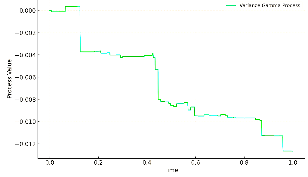
The plotted graph represents a simulation of the Variance Gamma (VG) process over a time horizon of 1 year, using specified parameters.

In this simulation, the VG process is characterized by:

• volatility parameter, σ=0.12
• rate of drift, ν=0.1
• drift of the Brownian motion part, θ=−0.14, and
• γ=0.2, controlling the variance of the gamma process.

The resulting path illustrates how the VG process can model asset price dynamics with jumps.

This reflects its utility in capturing the leptokurtosis and skewness observed in financial market returns.

Variance Gamma Process Solution

For example, this could represent:

• a managed exchange rate (where it’s periodically adjusted by policymakers)
• interest rate levels
• private asset valuations that are adjusted only occasionally
• certain types of derivatives

Conclusion

The Variance Gamma process sheds insight into the behavior of asset prices that are not captured by simpler models.

Its ability to model stochastic volatility and jumps makes it a valuable model for option pricing, risk management, and market analysis across different asset classes.