Statistical Moment Trading

Statistical Moment Trading is a quantitative trading strategy that leverages the mathematical concept of moments to analyze and predict market behavior.

It involves the use of various statistical moments to understand the distribution and characteristics of asset prices, which in turn helps traders make better decisions.

Mean-variance optimization is a classic approach to finance, but more modern approaches understand the shape and deeper characteristics of distributions – i.e., the skew and tailedness of the distribution rather than, for example, viewing volatility as a basic standard deviation.

Tail events can dramatically change the long-run performance of trading strategies, which makes understanding probability distributions and their moments important.

Key Takeaways – Statistical Moment Trading

• Capture Mean Reversion
  • Statistical moment trading focuses on concepts like mean reversion (allowing traders to profit from price deviations returning to the mean).
• Statistical Measures
  • Traders use moments like mean, variance, skewness, and kurtosis to identify trading opportunities and understand their distributions.
• Risk Management
  • By understanding statistical moments, traders can better optimize their portfolios.

Overview of Statistical Moments

Statistical moments are quantitative measures used to describe the shape and characteristics of a probability distribution.

The most commonly used moments in trading are the first four:

• mean
• variance
• skewness
• kurtosis

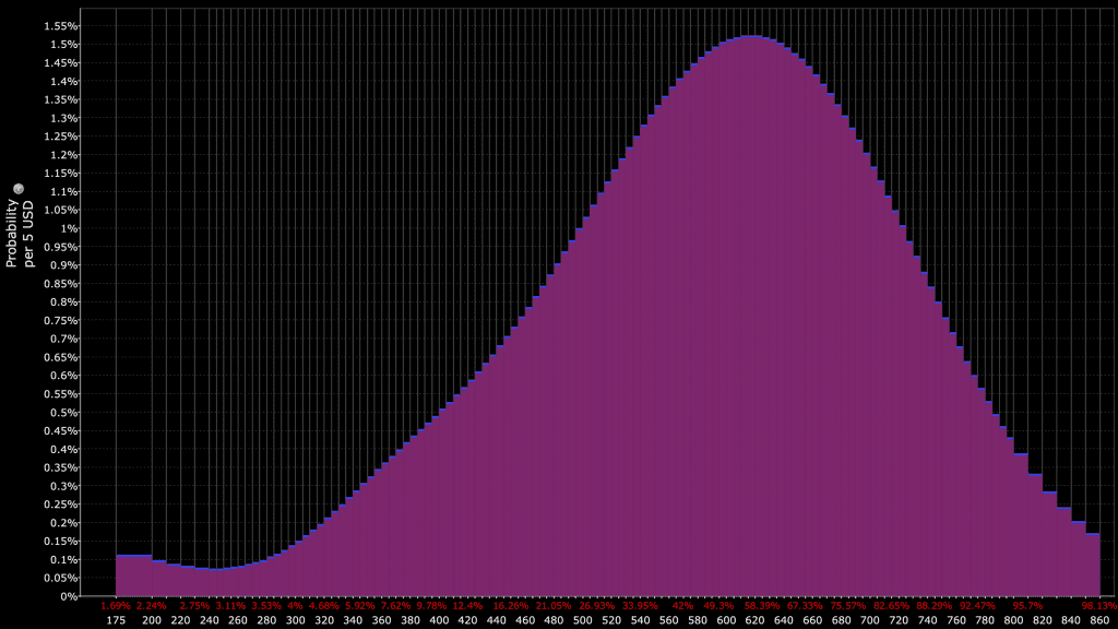
For normal distribution, skewness and kurtosis are zero. It’s the only distribution shape in which that’s true.

However, for financial return distributions, they will typically exhibit skew and fat tails (kurtosis), like the following:

Mean (First Moment)

The mean is the average of all data points in a distribution.

In trading, it represents the expected return of an asset.

By analyzing the mean, traders can identify the central tendency of price movements and make predictions about future price levels.

Variance (Second Moment)

Variance measures the dispersion of data points around the mean.

In the context of trading, variance indicates the volatility of an asset.

High variance suggests greater risk, as prices are more spread out, while low variance indicates more stable prices.

Skewness (Third Moment)

Skewness measures the asymmetry of the distribution.

Positive skewness indicates that the distribution has a long right tail, suggesting that there are frequent small losses and occasional large gains.

Negative skewness, on the other hand, indicates a long left tail, suggesting frequent small gains and occasional large losses.

Understanding skewness helps traders anticipate the direction and magnitude of potential price movements.

Kurtosis (Fourth Moment)

Kurtosis measures the “tailedness” of the distribution.

High kurtosis means the distribution has heavy tails and sharp peaks, indicating a higher likelihood of extreme price movements.

Low kurtosis indicates lighter tails and a flatter peak, suggesting fewer extreme price movements.

Traders use kurtosis to assess the risk of extreme market events.

Higher-Order Moments Beyond Kurtosis

Higher-order moments beyond the fourth moment provide deeper insights into the shape and behavior of a distribution.

They’re often used in more advanced statistical and financial analysis:

Fifth Moment (Fifth Cumulant)

Measures asymmetry and tail behavior.

Extends skewness by capturing more nuanced deviations from symmetry.

Sixth Moment (Sixth Cumulant)

Captures the extent and impact of extreme values, extending kurtosis by identifying more extreme outliers.

Seventh and Eighth Moments 

Rarely used but can provide further details on the distribution’s shape, focusing on more intricate aspects of asymmetry and tail behavior.

These higher-order moments are less commonly used due to their complexity and the diminishing practical utility in many real-world applications.

They can however be used in fields requiring precise risk assessment and modeling of extreme events, such as in certain areas of finance and insurance.

Application in Trading

Statistical moment trading applies these moments to create models that predict future price movements and volatility.

Here’s how each moment is used:

Mean Reversion

Traders using mean reversion strategies assume that asset prices will revert to their historical mean over time.

By identifying deviations from the mean, they can buy undervalued assets and sell overvalued ones, expecting prices to move back toward the mean.

Volatility Forecasting

Variance is used for forecasting volatility.

Traders analyze historical variance to predict future price fluctuations and adjust their trading strategies accordingly, and understand what structural changes have occurred that make future volatility likely to differ from historical volatility.

For instance, in high volatility environments, traders might reduce their position sizes to manage risk.

(Market makers will commonly widen bid-ask spreads.)

Skewness Analysis

From analyzing skewness traders can predict the direction of future price movements.

• Positive skewness indicates a distribution with an asymmetric tail extending toward more positive values.
• Negative skewness shows a distribution with an asymmetric tail going toward more negative values.

Tail Risk Management

Kurtosis is used to assess the risk of extreme market events.

High kurtosis suggests a higher probability of significant price changes, prompting traders to implement risk management strategies such as stop-loss orders or hedging (e.g., put options) to protect their portfolios.

Implementation Techniques

Statistical moment trading requires computational systems and techniques to analyze large datasets and calculate moments.

Common methods include:

Statistical Software

Traders often use statistical software like R, Python, and MATLAB to compute moments and perform data analysis.

These tools offer powerful libraries and functions for statistical modeling and visualization.

Machine Learning

Machine learning algorithms can enhance statistical moment analysis by identifying patterns and relationships that are not apparent through traditional methods.

Techniques such as regression analysis, clustering, and neural networks can be applied to improve predictive accuracy.

Real-Time Data

High-frequency trading platforms and APIs provide the necessary data feeds.

Advantages and Limitations

Advantages

• Precision – Statistical moments provide precise quantitative measures to improve the accuracy of trading models.
• Risk Management – Understanding the distribution characteristics of asset prices enables traders to better manage risk and avoid extreme losses.
• Versatility – The approach can be applied to various asset classes, including stocks, commodities, and currencies.
• Software – Many software packages (e.g., Python) are able to calculate the first four moments/cumulants (mean, variance, skew, kurtosis) of data.

Limitations

• Complexity – The mathematical and computational needs of statistical moment trading require expertise and resources.
• Data Dependency – The accuracy of moment calculations depends on the quality and completeness of historical data.
• Market Assumptions – The assumption that historical moments will predict future behavior may not always hold, especially when the future is different from the past.

Let’s look at some trades involving statistical moment trading:

Trade Example 1: Mean Reversion Strategy

Identify the Asset

Choose a stock, say XYZ Corp, currently trading at $100 per share.

Historical Data Analysis

Analyze the historical price data of XYZ Corp to determine the historical mean price.

Suppose the historical mean price is $95.

Deviation Identification

Identify the current deviation from the mean.

In this case, the stock is trading at $100, which is $5 above the historical mean.

Determine Entry Point

Set a threshold for deviation that signals a mean reversion trade.

Assume the threshold is $4.

Since the current price is $5 above the mean, it exceeds the threshold.

Place the Trade

Sell short 100 shares of XYZ Corporation at $100 per share, anticipating that the price will revert to the mean.

Monitor the Trade

Monitor the price movement.

Exit the Trade

Once the price reverts to the mean of $95, cover the short position by buying 100 shares at $95 per share.

Trade Details

• Entry Price: $100 per share
• Shares Sold Short: 100
• Exit Price: $95 per share
• Profit: (100 – 95) * 100 = $500

Trade Example 2: Volatility Forecasting

Identify the Asset

Choose an asset. Let’s call it ABC Futures.

Historical Variance Calculation

Calculate the historical variance of ABC Futures prices over a specific period.

Assume the variance is 0.04 (4%).

Forecast Future Volatility

Use the historical variance to forecast future volatility.

Suppose the forecasted variance for the next month is 0.05 (5%).

Determine Position Size

Adjust the position size based on the forecasted volatility.

If the usual position size is 10 contracts, reduce it by 20% due to increased forecasted volatility.

Place the Trade

Buy 8 ABC Futures Contracts instead of 10 to manage the risk associated with higher volatility.

Set Stop-Loss Orders

Place stop-loss orders or options to protect against adverse price movements.

For example, set a stop-loss at 2% below the entry price.

Trade Details

• Standard Position Size: 10 contracts
• Adjusted Position Size: 8 contracts
• Entry Price: Assume $1,000 per contract
• Stop-Loss Level: $980 per contract (2% below entry price)

Trade Example 3: Skewness Analysis

Skewness is a measure of the asymmetry of the probability distribution of returns for a given investment.

Interpreting Skewness

• Positive Skewness – Indicates potential for extreme positive returns, but fewer in frequency. A trader might see this as an opportunity for high upside.
• Negative Skewness – Indicates potential for extreme negative returns, suggesting a risk of significant losses. A trader might proceed with caution or hedge their positions.

Strategy Development

• Positive Skewness – Traders might opt for strategies that capitalize on the likelihood of positive tail events, such as buying out-of-the-money call options.
• Negative Skewness – Traders might implement risk management strategies like stop-loss orders or buying put options to protect against extreme negative moves.

Practical Example

• Suppose a trader analyzes a stock and finds a skewness of 0.8 (positively skewed). They might decide to take a long position, anticipating that the stock/asset has a higher probability of experiencing positive returns.
• Conversely, if the skewness was -0.5 (negatively skewed), they might choose to either avoid taking a long position or use protective puts/options to guard against potential large losses.

Trade Example 4: Tail Risk Management (Kurtosis)

Asset Choice

Choose an asset.

Historical Kurtosis Calculation

Find the expected kurtosis of the asset’s price distribution.

Assume the kurtosis is high, indicating a likelihood of extreme price movements.

Risk Management Strategy

Implement a strategy to hedge against potential extreme price movements.

Buy out-of-the-money (OTM) put options as insurance.

Determine Option Details

Choose OTM put options with a strike price 10% below the current price.

Assume the current price is $200 per share, so buy put options with a strike price of $180.

Place the Trade

Buy 10 put options contracts (each contract typically represents 100 shares) with a strike price of $180.

Monitor and Adjust

Adjust as necessary based on price movements and changes in kurtosis.

Trade Details

• Current Price: $200 per share
• Strike Price of Put Options: $180
• Number of Contracts: 10
• Cost per Option Contract: Assume $2 per share (total cost = 10 * 100 * $2 = $2,000)

Conclusion

Statistical moment trading is a strategy that leverages the mathematical properties of distributions to improve trading decisions.

By understanding and applying the concepts of mean, variance, skewness, and kurtosis (and potentially higher-order moments beyond that), traders can gain deeper insights into the nature of their expected returns and better learn to optimize their portfolios – or at least be aware of certain risks.