Random Matrix Theory in Finance & Trading

Random Matrix Theory (RMT) is a statistical framework used to analyze the properties of matrices with random elements.

In finance and trading, RMT is useful for analyzing the structure of correlations among assets in large portfolios, which can help with understanding why assets move the way they do, risk management, and portfolio optimization.

Key Takeaways – Random Matrix Theory in Finance & Trading

• Noise Reduction
  • Random Matrix Theory (RMT) helps distinguish genuine correlations in financial data from noise.
  • By analyzing the eigenvalues of correlation matrices, traders can identify stable relationships between assets and ignore random fluctuations
    • Improves portfolio optimization.
• Portfolio Diversification
  • RMT guides the construction of more diversified portfolios by revealing the inherent structure of correlations among assets.
  • This insight allows traders to select assets that genuinely offer diversification benefits – reducing risk without sacrificing returns.
• Risk Management
  • By understanding the limitations of correlation matrices (including the stability and significance of correlations), traders can better manage systemic risk.
  • RMT provides a framework to evaluate market stability and potential for extreme co-movements to improve risk assessment strategies.

Here are some key concepts and applications of RMT in finance and trading:

Key Concepts of RMT in Finance

Eigenvalues & Eigenvectors

In the context of financial correlation matrices, eigenvalues represent the variance explained by each eigenvector, which corresponds to a specific pattern of asset returns.

RMT helps distinguish between eigenvalues that arise from true financial asset correlations and those that result from noise.

Marchenko-Pastur Law

This law provides a theoretical distribution of eigenvalues for a random correlation matrix.

It helps identify:

• which eigenvalues in a financial correlation matrix are statistically significant, and
• which are likely due to random noise

Noise Reduction

RMT is used to filter out noise in empirical correlation matrices.

By identifying the eigenvalues that are outside the bounds predicted by the Marchenko-Pastur Law, analysts can isolate the signal (true underlying correlations) from the noise (random fluctuations).

Random Matrix Theory Applications for Traders

Portfolio Optimization

RMT can improve the Markowitz portfolio optimization framework by filtering out noise in the correlation matrix of asset returns.

This leads to more stable and reliable estimates of risk and return.

This can help traders and portfolio managers construct more efficient portfolios.

Risk Management

By identifying the principal components of a portfolio’s risk structure (through eigenvector analysis), traders can better understand their exposures to systematic risk factors.

This allows for more targeted risk mitigation strategies, such as hedging against specific risk factors.

Market Structure Analysis

RMT can be used to analyze the market structure, identifying periods of high correlation among stocks versus periods when individual stock performance is more idiosyncratic.

This information can be used for strategies that depend on diversification to reduce risk.

Identifying Stable Correlations

In financial markets, correlations between assets can change over time.

For example, here’s the 36-month rolling correlation of SPY (S&P 500 ETF) and TLT (long-duration US Treasury bond ETF):

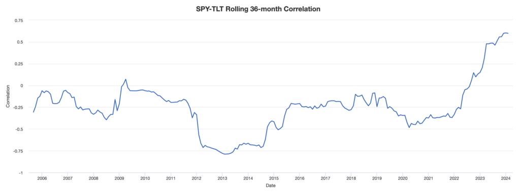
You can see that this correlation changes significantly – and also depends on the timeframe it’s measured.

There’s what assets are intrinsically like (which itself can change over time), and then there’s the environment they’re in, which causes them to perform in different ways.

This, in turn, impacts their correlations over time.

RMT helps traders identify the most stable correlations, which are important for long-term trading/investment strategies and for understanding fundamental relationships between assets.

Stress Testing and Scenario Analysis

By understanding the underlying structure of asset correlations, traders can better simulate extreme market conditions and assess the potential impact on their portfolios.

This is often done by generating synthetic data (since many hypothetical events haven’t occurred before and so no backtesting is available).

This is important for developing strong risk management strategies that can withstand any type of market.

Implementation Considerations

Data Requirements

Implementing RMT in finance requires access to high-quality financial data, including prices, returns, and other relevant market data.

Computational Complexity

The analysis involves complex mathematical and statistical computations.

This requires both expertise and computational resources.

Dynamic Markets

Financial markets are dynamic, and the stability of correlations can vary over time.

Traders must continuously update their models to reflect changing market conditions.

Coding Example – Random Matrix Theory

Using a portfolio we’ve used in many other examples, let’s say we wanted to develop some Python code to help understand how to optimize this portfolio using Random Matrix Theory.

• Stocks: +3-7% forward return, 15% annualized volatility using standard deviation
• Bonds: +1-5% forward return, 10% annualized volatility using standard deviation
• Commodities: +0-4% forward return, 15% annualized volatility using standard deviation
• Gold: +2-6% forward return, 15% annualized volatility using standard deviation

import numpy as np
import matplotlib.pyplot as plt
from scipy.optimize import minimize

# Define expected return rates & volatilities
assets = ['Stocks', 'Bonds', 'Commodities', 'Gold']
returns = np.array([0.05, 0.03, 0.02, 0.04]) # Average forward returns for Stocks, Bonds, Commodities, Gold
volatilities = np.array([0.15, 0.10, 0.15, 0.15]) # Annualized volatilities

# Synthetic correlation matrix for demonstration
# In practice, should be derived from historical data or RMT methods
np.random.seed(71) 
random_correlations = np.random.rand(4, 4)
correlation_matrix = np.triu(random_correlations, 1)
correlation_matrix += correlation_matrix.T # Make the matrix symmetric
np.fill_diagonal(correlation_matrix, 1) # Fill the diagonal with 1s for self-correlation

# Convert correlation matrix to covariance matrix
covariance_matrix = np.outer(volatilities, volatilities) * correlation_matrix

# Define portfolio optimization problem
def portfolio_variance(weights, cov_matrix):
return weights.dot(cov_matrix).dot(weights)

def portfolio_return(weights, returns):
return np.sum(weights * returns)

def objective_function(weights, cov_matrix, returns, risk_aversion=0.5):
return -portfolio_return(weights, returns) + risk_aversion * portfolio_variance(weights, cov_matrix)

# Constraints: sum of weights = 1
constraints = ({'type': 'eq', 'fun': lambda x: np.sum(x) - 1})

# Bounds for weights
bounds = tuple((0, 1) for asset in assets)

# Initial guess (equal allocation)
initial_guess = np.array([0.25, 0.25, 0.25, 0.25])

# Optimize
result = minimize(objective_function, initial_guess, args=(covariance_matrix, returns), method='SLSQP', bounds=bounds, constraints=constraints)

# Print optimized weights
optimized_weights = result.x
print("Optimized Portfolio Weights:")
for asset, weight in zip(assets, optimized_weights):
print(f"{asset}: {weight:.2%}")

# Plotting
plt.figure(figsize=(10, 6))
plt.bar(assets, optimized_weights, color='skyblue')
plt.title('Optimized Portfolio Allocation Using Random Matrix Theory (Synthetic Example)')
plt.xlabel('Asset')
plt.ylabel('Allocation')
plt.show()

Explanation

This Python code optimizes a portfolio of stocks, bonds, commodities, and gold based on expected returns, volatilities, and a synthetic correlation matrix.

It minimizes a risk-adjusted objective function that balances expected returns against portfolio variance.

Constraints ensure the portfolio weights sum to 1.

Tensors in the Context of Random Matrix Theory

Tensors are generalizations of scalars, vectors, and matrices to higher dimensions.

• A scalar is a zero-dimensional tensor
• A vector is a one-dimensional tensor, and
• A matrix is a two-dimensional tensor

Tensors of higher dimensions (three-dimensional and beyond) are used to represent multidimensional data.

In finance and trading, the underlying principles of tensor analysis and matrix theory are indeed applicable, especially in areas such as:

Multivariate Time Series Analysis

High-dimensional financial data, such as prices of multiple assets over time, can be modeled using tensors to capture the dynamic relationships between different market variables.

Portfolio Optimization

Tensors can represent the covariances among multiple assets across different times.

Allows for more sophisticated models of risk and return that account for the temporal dynamics of financial markets.

Machine Learning and Artificial Intelligence

Tensors are central to the operations of deep learning algorithms, which are increasingly used in algorithmic trading and quantitative finance to predict market movements and optimize trading strategies.

Complex Derivatives Pricing

In models for pricing complex derivatives, tensors can represent the sensitivities of an instrument’s price to changes in underlying factors, which extends beyond the simple matrix representations used in basic options pricing models.

The mathematical concepts of tensors and matrices are embedded in the quantitative methods used in these fields.

These tools help deal with the complexity of financial markets, which enable traders and analysts to model, analyze, and make predictions about market behavior with greater accuracy.

Conclusion

Random Matrix Theory provides a way to analyze correlations in financial markets.

This can help traders and portfolio managers make more informed decisions about portfolio construction, risk management, and market analysis.

At the same time, the application of RMT requires a deep understanding of both the theory and the practical realities of financial markets.