Neutral Rate – Why Is It Important?


The neutral rate is the level of interest rates – often referring to a short-term overnight rate – that neither stimulates nor restrains economic activity.
When policy rates are considered near neutral, the economy is expected to grow close to its long run potential with inflation remaining stable.
The neutral rate is fundamentally a reference point, not a fixed number.
It moves over time as productivity, demographics, spending, and global capital flows change.
In this article, we’ll take a look at why various market participants and entities care and how to estimate it.
Key Takeaways – Neutral Rate
- The neutral rate is the interest rate that neither stimulates nor restrains the economy.
- When policy is near neutral, growth is near potential and inflation is stable.
- Neutral is a moving reference point rather than a fixed number.
- It shifts with productivity, demographics, spending patterns, and global capital flows.
- Central banks use it to judge whether policy is restrictive (tight) or accommodative (loose).
- Markets use it to anchor long run expectations for yields, valuations, and currencies.
- Changes in perceived neutral can reprice assets even without rate moves.
- For example, a lower neutral rate will tend to push risk assets like equities higher because shorter-duration assets now yield less.
- A higher neutral rate leads to less inflows into equities, as it increases the hurdle rate for equity returns and the opportunity cost of holding stocks isn’t as high.
- The neutral rate shapes the baseline return environment for portfolios.
- Higher neutral implies higher yields and lower valuation multiples.
- Lower neutral implies lower yields and higher sensitivity to rate changes because the duration of assets structurally lengthens.
- Neutral is unobservable and uncertain, so like many things in finance, it’s more of a range/distribution rather than precision.
Why Does the Neutral Rate Matter?
Why Central Banks Care
Central banks use the neutral rate as a benchmark for policy stance.
If the policy rate is above neutral, monetary policy is restrictive and intended to slow growth, generally with the central goal of reining in inflation.
If it’s below neutral, policy is accommodative and intended to support growth and pulling workers off the sidelines so the economy can reach its full output potential.
Without an estimate of neutral (a range is fine and appropriate), policymakers lack context for whether rates are tight or loose.
Why Markets Care
For investors/traders, the neutral rate anchors long run expectations for interest rates, bond yields, and discount rates.
It influences equity valuations, term premia (the relative yield differentials between bond), and currency trends.
Shifts in perceived neutral can reprice assets even without immediate policy changes.
Why It Matters for Portfolio Construction
The neutral rate shapes the baseline return environment.
It’s the cash rate (i.e., short-term bonds), which helps set pricing in longer-duration instruments.
A higher neutral rate implies structurally higher yields but lower valuation multiples.
A lower neutral rate implies lower yields, higher sensitivity to rate changes (the duration of assets lengthens), and can create a greater reliance on diversification and alternatives.
Key Limitation
The neutral rate is unobservable and uncertain.
Different models and market participants disagree, which is why markets react strongly when expectations about neutral change rather than when it’s precisely estimated.
How Traders View It
The neutral rate is important because it’s the most fundamental building block of asset returns.
The risk-free return is typically the return on cash, though it should be whatever rate best/effectively neutralizes your risks.
For example, for investors or traders looking for real (inflation-adjusted) returns, the risk-free return is the return on inflation-indexed bonds).
The return from betas is lowered on top of the risk-free rate, which is what we call a risk premium.
A 10-year bond typically has a risk premium over the cash rate because you want to get paid for taking the extra duration risk.
And corporate bonds have a risk on top of that because there’s credit risk, holding duration constant.
Equities contain credit and duration risk, and you generally expect compensation in excess of bonds, with the duration theoretically perpetual. In other words, there’s no expiration date, unlike most forms of bonds.
You can observe their relative risk premiums by roughly looking at the differences in their returns over long stretches of time.
For example, since 1974:
Portfolio Assets
| Name | CAGR | Stdev | Best Year | Worst Year | Max Drawdown | Sharpe Ratio | Sortino Ratio |
|---|---|---|---|---|---|---|---|
| US Stock Market | 11.38% | 15.69% | 37.82% | -37.04% | -50.89% | 0.49 | 0.71 |
| 10-year Treasury | 6.41% | 8.12% | 39.57% | -15.19% | -23.18% | 0.26 | 0.41 |
| Long-Term Corporate Bonds | 7.28% | 8.85% | 28.68% | -25.62% | -33.85% | 0.34 | 0.52 |
| Cash | 4.50% | 1.00% | 15.29% | 0.03% | 0.00% | -0.15 | -0.18 |
| Gold | 7.08% | 18.76% | 126.55% | -32.60% | -61.78% | 0.22 | 0.35 |
Let’s look at the relative risk premiums.
Naturally, these are not set in stone and even despite 50+ years of history, they can vary over time.
US Stocks vs Cash: +6.9% annual risk premium
Stocks (11.38%) minus cash (4.50%).
This is the classic equity risk premium for bearing volatility and drawdowns.
US Stocks vs 10-Year Treasuries: +5.0% risk premium
Compensation for higher volatility, deeper drawdowns, and cyclical risk.
US Stocks vs Long-Term Corporate Bonds: +4.1% risk premium
Reflects additional equity risk beyond credit and duration risk.
Long-Term Corporate Bonds vs Treasuries: +0.9% credit risk premium
Extra return for taking default risk and spread volatility.
Treasuries vs Cash: +1.9% duration risk premium
Compensation for interest rate sensitivity versus capital stability.
Gold vs Cash: +2.6% alternative risk premium
Return comes with high volatility and large drawdowns, not income.
Gold vs Treasuries: +0.7% volatility premium
Modest excess return.
Gold vs US Stocks: –4.3% relative return gap
Gold underperformed equities long term.
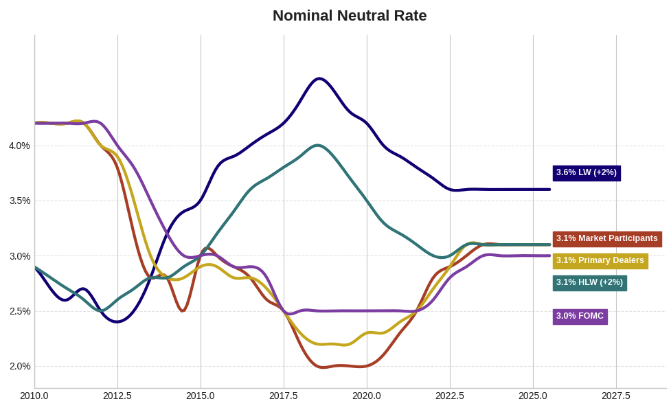
Nominal Neutral Rate Estimates and Survey Measures
LW (+2%)
LW refers to the Laubach-Williams estimate of the neutral real interest rate (r-star, r*), adjusted to a nominal rate by adding 2% as a long-run inflation assumption.
This is a structural macroeconomic model that estimates the real policy rate consistent with stable inflation and output near potential.
It’s not a policy target, but an analytical benchmark.
For those interested in how this is calculated, we’ve included that in the Appendix to this article.
HLW (+2%)
HLW stands for Holston-Laubach-Williams, an updated and refined version of the original LW model, again converted to a nominal rate by adding 2% inflation.
It provides an alternative model-based estimate of r* that incorporates additional data and methodological improvements, often cited in Fed research and policy discussions.
HLW keeps the same economic structure as LW but improves estimation.
Calculations and an example are in the Appendix.
FOMC
FOMC is the monetary policy body of the Federal Reserve. They consist of the Board of Governors and regional Federal Reserve Bank presidents.
There are 12 voting members.
This committee sets the federal funds rate target range and conducts US monetary policy.
In this context, the FOMC line reflects the committee’s long-run nominal policy rate projection from the Summary of Economic Projections.
Primary Dealers
Primary Dealers are official counterparties to the New York Fed in open market operations.
They’re a select group of large banks and broker-dealers designated by the Federal Reserve Bank of New York.
They underwrite US Treasury issuance, make markets in government securities, trade directly with the Fed, and submit formal forecasts on growth, inflation, and interest rates through Fed surveys.
Primary dealers are eligible to participate in specific Fed lending facilities, such as the Standing Repo Facility (SRF) and the Overnight Reverse Repurchase Agreement (ON RRP) Facility.
Market Participants
Market participants refers to a broader investor survey group beyond primary dealers.
Includes asset managers, hedge funds, pension funds, insurance companies, banks, and other major institutional investors.
Provide expectations-based forecasts that reflect how financial markets interpret economic conditions and the likely long-run level of interest rates.
This image gives an idea of how each has estimated the nominal neutral rate since 2010:
Appendix
How the LW (+2%) Model is Calculated
Core Objects Estimated
- r_star_t = neutral real interest rate
- y_star_t = potential output
- g_t = trend growth rate
- pi_t = inflation
- i_t = nominal policy rate
- y_gap_t = output gap = y_t − y_star_t
IS Curve (Aggregate Demand)
y_gap_t = a1 * y_gap_(t−1) + a2 * (i_t − pi_t − r_star_t) + e_y_t
This says output depends on:
- past output gaps
- how restrictive policy is relative to neutral
Phillips Curve (Inflation)
pi_t = b1 * pi_(t−1) + b2 * y_gap_t + e_pi_t
Inflation responds to economic slack.
Potential Output Growth
y_star_t = y_star_(t−1) + g_t + e_y*_t
Trend Growth (Random Walk)
g_t = g_(t−1) + e_g_t
Neutral Real Rate Definition
r_star_t = c * g_t + z_t
Where:
- g_t = trend productivity growth
- z_t = other slow-moving structural factors (demographics, savings, global capital flows)
Nominal Neutral Rate (what’s plotted)
r_star_nominal_t = r_star_t + 0.02
The +2% is a long-run inflation assumption, not estimated inside the model.
How the HLW (+2%) Model is Calculated
Key Differences in Inputs
- Uses multiple countries (US, euro area, UK, Canada)
- Better filtering of trend growth and output gaps
- Better treatment of unobserved components
Neutral Rate (Same Functional Form)
r_star_t = c * g_t + z_t
But:
- g_t and z_t are estimated with cross-country information
- Lower model instability than LW
Nominal Neutral Rate
r_star_nominal_t = r_star_t + 0.02
Again, 2% is an external inflation anchor, not a model output.
Important Clarifications
- There is no single closed-form equation for r*
- r* is inferred jointly from:
- GDP
- Inflation
- Interest rates
- GDP
- LW and HLW are Kalman-filtered state space models
- Outputs are estimates with wide confidence bands
Practical Interpretation
- LW and HLW estimate where policy should converge over the long run
- Adding +2% converts a real equilibrium rate into a nominal policy benchmark
- Markets care more about changes in r* than its absolute level
So, let’s do some example calculations of each:
LW (+2%) Example Calculations (Illustrative Numbers)
Assume the following coefficients and inputs for one period t:
- a1 = 0.60, a2 = -0.50
- b1 = 0.70, b2 = 0.40
- c = 1.00
- y_gap_(t−1) = 1.00%
- i_t = 4.50% (nominal policy rate)
- pi_t = 2.50% (inflation)
- pi_(t−1) = 2.30%
- y_star_(t−1) = 100.00 (index level)
- g_(t−1) = 1.50%
- e_y_t = 0.10%, e_pi_t = 0.00%, e_y*_t = 0.05, e_g_t = 0.10%
- z_t = 0.30% (slow moving factor)
1) Trend Growth (Random Walk)
g_t = g_(t−1) + e_g_t
g_t = 1.50% + 0.10% = 1.60%
2) Neutral Real Rate Definition
r_star_t = c * g_t + z_t
r_star_t = 1.00 * 1.60% + 0.30% = 1.90%
3) Real Policy Rate Gap (Restrictiveness Term)
(i_t − pi_t − r_star_t) = 4.50% − 2.50% − 1.90% = 0.10%
Interpretation: policy is 0.10% above neutral in real terms (slightly restrictive).
4) IS Curve (Output Gap)
y_gap_t = a1 * y_gap_(t−1) + a2 * (i_t − pi_t − r_star_t) + e_y_t
y_gap_t = 0.60 * 1.00% + (−0.50) * 0.10% + 0.10%
y_gap_t = 0.60% − 0.05% + 0.10% = 0.65%
5) Phillips Curve (Inflation)
pi_t = b1 * pi_(t−1) + b2 * y_gap_t + e_pi_t
pi_t = 0.70 * 2.30% + 0.40 * 0.65% + 0.00%
pi_t = 1.61% + 0.26% = 1.87%
(If actual observed inflation is 2.50% in your data, the model errors would absorb that difference.)
6) Potential Output Growth
y_star_t = y_star_(t−1) + g_t + e_y*_t
If y_star is an index and g_t is a percent growth rate, convert to levels:
Growth contribution = 100.00 * 1.60% = 1.60
y_star_t = 100.00 + 1.60 + 0.05 = 101.65
7) Nominal Neutral Rate (What’s Plotted)
r_star_nominal_t = r_star_t + 0.02
r_star_nominal_t = 1.90% + 2.00% = 3.90%
That “3.90%” is the LW (+2%) nominal neutral estimate for this illustrative period.
HLW (+2%) Example Calculations (Same Structure, Different Inputs)
HLW uses the same functional form but estimates g_t and z_t using cross-country data, which can change the implied neutral rate materially.
Assume HLW cross-country filtering produces:
- g_t = 1.20% (lower trend growth)
- z_t = 0.10% (lower structural component)
- c = 1.00
1) Neutral Real Rate (HLW)
r_star_t = c * g_t + z_t
r_star_t = 1.00 * 1.20% + 0.10% = 1.30%
2) Nominal Neutral Rate (HLW +2%)
r_star_nominal_t = r_star_t + 0.02
r_star_nominal_t = 1.30% + 2.00% = 3.30%
3) Policy Restrictiveness vs HLW Neutral (Optional but Useful)
(i_t − pi_t − r_star_t) = 4.50% − 2.50% − 1.30% = 0.70%
Interpretation: policy is 0.70% above neutral in real terms (more restrictive than in the LW example).
What These Examples Demonstrate
LW and HLW differ mainly because they can estimate g_t (trend growth) and z_t (structural component) differently.
Adding +2% is just a conversion from a real neutral rate to a nominal benchmark.
As mentioned, the model is typically estimated with a Kalman filter, so in practice these calculations happen jointly across time with measurement errors and uncertainty bands.