Hierarchical Risk Parity (A ML Approach to Building Balanced and Well-Diversified Portfolios)

Key Takeaways – Hierarchical Risk Parity

• Hierarchical Risk Parity (HRP) is a portfolio optimization method focused on allocating assets based on their risk contributions to provide a more balanced and diversified portfolio.
• HRP uses hierarchical clustering and risk parity principles to construct portfolios. This allows for better risk management and adaptability to changing market conditions.
• HRP’s focus on risk contributions reduces its susceptibility to estimation errors, potentially leading to more consistent results over time.
• While HRP offers several advantages over traditional methods like Modern Portfolio Theory (MPT), it’s important to consider individual goals and risk tolerance when evaluating its suitability for your investment needs.
• We do a Python example below.

Hierarchical Risk Parity vs. Risk Parity

Hierarchical Risk Parity (HRP) and Traditional Risk Parity (RP) are two approaches to portfolio construction that aim to optimize the allocation of assets based on their risk contributions.

Nonetheless, they differ significantly in their methodologies and underlying assumptions.

Traditional Risk Parity (RP)

Equal Risk Contribution

RP aims to allocate assets in such a way that each asset contributes equally to the portfolio’s overall risk.

This is usually measured in terms of volatility or variance.

Correlation and Covariance

RP relies on the correlation and covariance matrix of the asset returns to determine the asset weights.

Assumption

Many RP approaches assume that the historical correlations and volatilities will remain relatively stable over the investment horizon.

Challenges

One challenge with RP is its sensitivity to the estimation of correlations and volatilities.

This can lead to significant changes in asset allocation with small changes in these parameters.

Hierarchical Risk Parity (HRP)

Cluster-Based Approach

HRP is a more sophisticated approach that first clusters assets based on their price movements and then applies risk parity within and across these clusters.

Hierarchy and Tree Structures

HRP uses a hierarchical tree (dendrogram) to understand the structure of asset correlations.

Assets are grouped into clusters with similar price behavior, and then these clusters are themselves clustered, creating a tree-like structure.

Less Sensitivity to Estimation Errors

Since HRP doesn’t solely rely on the covariance matrix, it tends to be less sensitive to estimation errors in correlations and volatilities.

Intuitive and Adaptive

HRP is considered more intuitive and adaptive to changing market conditions, as it recognizes the inherent structure in asset movements.

Summary

Traditional risk parity focuses on equalizing risk contribution based solely on volatility and correlation.

HRP takes a more nuanced approach by recognizing the hierarchical structure in asset correlations and can be further tailored by incorporating various constraints (which we discuss in the next section).

Hierarchical Risk Parity with Constraints

Incorporating Constraints

HRP can be adapted to include various constraints, such as maximum or minimum weights on certain assets, sector constraints, liquidity considerations, or regulatory requirements.

Customization for Specific Goals

By adding constraints, investors can tailor the HRP model to specific investment goals or risk management requirements.

Complexity in Optimization

The inclusion of constraints adds complexity to the optimization process.

It requires more sophisticated mathematical techniques to ensure that the portfolio adheres to the constraints while still maintaining the benefits of the HRP approach.

Potential for Enhanced Performance

If properly implemented, HRP with constraints can potentially lead to enhanced performance and risk management.

It allows for a more tailored approach to portfolio construction that aligns with specific trading/investment objectives or regulatory requirements.

While Hierarchical Risk Parity (HRP) offers several advantages as a portfolio optimization method, it’s important to recognize its potential limitations.

Changing Correlations: The Non-Static Nature

One significant drawback of many approaches to HRP is its reliance on historical correlations between assets.

Correlations are not static and can change over time, making it challenging to predict future relationships based on past data.

Relying on historical correlations can lead to an over- or underestimation of the actual risk in the portfolio.

When a bunch of data is fed into the computer and this spits out algorithms for dealing with the future, this is often known as overfitting.

When the past is different from the future and the past is what those algorithms are based on, this can be very risky.

Moreover, during periods of market stress or significant shifts in market conditions, correlations between assets can change rapidly.

In such cases, HRP’s often backward-looking approach to constructing portfolios may not provide adequate protection against changing correlations, potentially leading to a less diversified and more vulnerable portfolio.

Instead, correlations are best known in the form of what fundamentally drives an asset’s pricing and movement.

Ideally, you’re looking for returns streams that are uncorrelated to each other.

And you can even do better than that through negatively correlated assets.

Overemphasis on Clustering

HRP’s reliance on hierarchical clustering can be both a strength and a weakness.

While clustering can help identify and group assets with similar risk profiles, it may also lead to an overemphasis on certain clusters or sectors.

This could result in under-diversification within the clusters themselves, potentially leading to increased vulnerability to sector-specific risks or market shifts.

Applicability in Certain Market Conditions

HRP may not be as effective during periods of significant market shifts or structural changes if the approach is heavily backward-looking, as its reliance on historical risk contributions might not always be indicative of future risk.

In such situations, the HRP approach might not provide adequate diversification, leaving the portfolio exposed to potential losses.

Hierarchical Risk Parity in Python – Clustering Example

Let’s first simulate a basic hierarchy, then show it visually.

We’ll do it this way:

• Equity Sectors cluster first
• Corporate Credit joins the equity cluster
• Nominal Government Bonds join next
• Inflation-Linked Government Bonds follow
• Gold joins thereafter
• Commodities join last

Here’s how we can simulate this in Python:

import numpy as np
import matplotlib.pyplot as plt
from scipy.cluster.hierarchy import dendrogram, linkage

# Manually define the asset classes in the desired hierarchical order
assets = [
    'Technology', 'Healthcare', # Equity Sectors
    'High Yield Credit', 'Investment Grade Credit', # Corporate Credit
    'Nominal Bonds', # Nominal Government Bonds
    'Inflation-Linked Bonds', # Inflation-Linked Government Bonds
    'Gold', # Gold
    'Commodities'# Commodities
]

# Manually create a linkage matrix to reflect the desired hierarchy
# The numbers here are fabricated to demonstrate the hierarchy and do not represent actual distances or metrics
link = np.array([
    [0, 1, 0.1, 2], # Technology and Healthcare cluster first
    [2, 3, 0.2, 2], # High Yield Credit and Investment Grade Credit cluster
    [4, 5, 0.3, 4], # The above two clusters join
    [6, 7, 0.4, 5], # Nominal Bonds join
    [8, 9, 0.5, 6], # Inflation-Linked Bonds join
    [10, 11, 0.6, 7], # Gold joins
    [12, 13, 0.7, 8], # Commodities join last
])

# Plot the dendrogram
plt.figure(figsize=(10, 7))
dendrogram(link, labels=assets, leaf_rotation=90)
plt.title("Hierarchical Clustering of Asset Classes")
plt.show()

# Get the order of assets according to the hierarchical tree
# Normally, leaves_list would be used here, but given the manual nature of 'link', we already have the order in 'assets'
sorted_assets = assets

# Display the sorted assets
print("Sorted Assets according to Hierarchy:")
print(sorted_assets)

Results

In this example, the linkage matrix (link) is manually constructed to demonstrate the hierarchy.

Each row in the matrix represents a merge between clusters, with the first two values being the indices of the clusters/leaves being merged, the third value being the distance (or dissimilarity) between these clusters, and the fourth value being the number of original observations in the newly formed cluster.

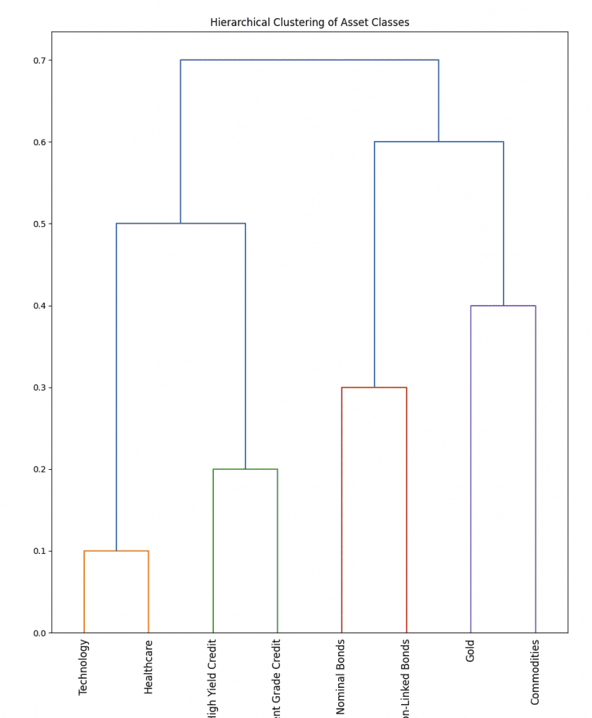
This structure is purely illustrative and serves to demonstrate how the assets would be arranged hierarchically.

In a real-world application, the linkage matrix would be derived from the data using clustering algorithms.

Simulate Hierarchical Clustering Algorithms

To perform hierarchical clustering on the specified asset classes, we typically use their historical return data to compute a distance or similarity measure (like correlation or covariance). 

Since we’re being illustrative in this context, we’ll use synthetic data here and we’ll simulate the process as if we had such data, allowing us to use a clustering algorithm to generate a linkage matrix.

 We’ll then compare it with the manually specified hierarchy in the link array.

Given asset classes:

• Technology
• Healthcare
• High Yield Credit
• Investment Grade Credit
• Nominal Bonds
• Inflation-Linked Bonds
• Gold
• Commodities

We will simulate returns for these assets and apply hierarchical clustering:

import numpy as np
import pandas as pd
from scipy.cluster.hierarchy import dendrogram, linkage
import matplotlib.pyplot as plt

# Asset classes
assets = [
    'Technology', 'Healthcare',
    'High Yield Credit', 'Investment Grade Credit',
    'Nominal Bonds',
    'Inflation-Linked Bonds',
    'Gold',
    'Commodities'
]

# Simulate some return data for these assets
np.random.seed(68)
num_days = 1000
returns = np.random.normal(0, 1, size=(num_days, len(assets)))

# Create a DataFrame for the returns
returns_df = pd.DataFrame(returns, columns=assets)

# Compute the correlation matrix, which will serve as our basis for clustering
correlation_matrix = returns_df.corr()

# Perform hierarchical clustering
linkage_matrix = linkage(correlation_matrix, method='ward')

# Plot the dendrogram
plt.figure(figsize=(12, 8))
dendrogram(linkage_matrix, labels=assets, leaf_rotation=90)
plt.title("Hierarchical Clustering of Asset Classes")
plt.xlabel("Asset Classes")
plt.ylabel("Distance")
plt.show()

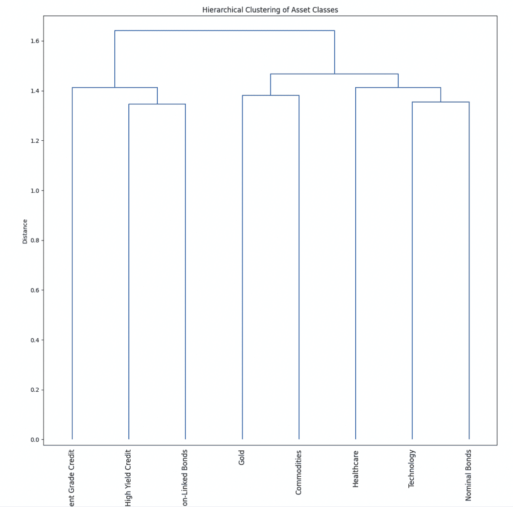
To sum what we did in this code:

• Simulate daily returns for each asset class to mimic real-world data.
• Compute the correlation matrix from these returns, which reflects how the assets move relative to each other.
• We use this correlation matrix as input to the linkage function, with the ‘ward’ method, to perform hierarchical clustering.
• The dendrogram visually represents the results. This shows how assets cluster together based on their simulated return patterns.

This process mimics how you’d typically perform hierarchical clustering in a financial context – i.e., by using historical returns data to inform the structure of the portfolio and understand the relationships between different asset classes. 

The ‘ward’ method minimizes the variance when forming clusters, aiming to form internally consistent but distinct clusters.

Results

Hierarchical Risk Parity in Python – Portfolio Weighting Example

To go off what we did in the above section, let’s weight an actual portfolio using hierarchical risk parity principles.

To simulate a logical covariance matrix for the asset classes with specific volatility characteristics and then estimate their relative weightings in a portfolio, we can follow these steps:

Define Volatilities

Assign a volatility value to each asset class, respecting the relative volatility characteristics (e.g., high yield (HY) credit more volatile than investment grade (IG) credit, etc.).

Simulate Correlations

Define logical correlations between asset classes.

Construct Covariance Matrix

Use the volatilities and correlations to construct a covariance matrix.

Portfolio Optimization

Use the covariance matrix to estimate relative weightings in the portfolio, assuming we aim to minimize portfolio variance.

Code

import pandas as pd
import numpy as np

# Annualized volatilities (in percentage)
volatilities = {
    'Technology': 20,
    'Healthcare': 14,
    'High Yield Credit': 12,
    'Investment Grade Credit': 10,
    'Nominal Bonds': 9,
    'Inflation-Linked Bonds': 8,
    'Gold': 15,
    'Commodities': 16
}

correlations = pd.DataFrame(
    [[1.00, 0.75, 0.30, 0.25, 0.10, 0.05, 0.20, 0.50], # Technology
    [0.75, 1.00, 0.25, 0.20, 0.15, 0.10, 0.15, 0.45], # Healthcare
    [0.30, 0.25, 1.00, 0.80, 0.40, 0.35, 0.25, 0.60], # High Yield Credit
    [0.25, 0.20, 0.80, 1.00, 0.45, 0.40, 0.20, 0.55], # Investment Grade Credit
    [0.10, 0.15, 0.40, 0.45, 1.00, 0.90, 0.10, 0.20], # Nominal Bonds
    [0.05, 0.10, 0.35, 0.40, 0.90, 1.00, 0.15, 0.25], # Inflation-Linked Bonds
    [0.20, 0.15, 0.25, 0.20, 0.10, 0.15, 1.00, 0.70], # Gold
    [0.50, 0.45, 0.60, 0.55, 0.20, 0.25, 0.70, 1.00]], # Commodities
    columns=volatilities.keys(), index=volatilities.keys()
)

# Convert annualized volatilities to standard deviations
std_devs = {k: v / 100 for k, v in volatilities.items()}

# Construct the covariance matrix
cov_matrix = pd.DataFrame(
    data=np.zeros((len(correlations), len(correlations))),
    columns=correlations.columns,
    index=correlations.index
)

for asset_i in cov_matrix.columns:
    for asset_jincov_matrix.index:
        cov_matrix.loc[asset_i, asset_j] =correlations.loc[asset_i, asset_j] *std_devs[asset_i] *std_devs[asset_j]
from scipy.optimize import minimize

# Define the objective function for optimization (portfolio variance)
def portfolio_variance(weights, covariance_matrix):
    return weights.T @covariance_matrix@weights

# Initial guess for weights
initial_weights = np.array(len(volatilities) * [1 / len(volatilities)])

# Constraints: sum of weights = 1
constraints = ({'type': 'eq', 'fun': lambda weights: np.sum(weights) - 1})

# Boundaries: weights between 0 and 1
bounds = tuple((0, 1) for asset in range(len(volatilities)))

# Perform optimization
result = minimize(
portfolio_variance,
initial_weights,
args=(cov_matrix,),
method='SLSQP',
bounds=bounds,
constraints=constraints
)

# Display the optimized weights

optimized_weights = pd.Series(result.x, index=cov_matrix.columns)
print("Optimized Portfolio Weights:")
print(optimized_weights)

Here, we:

• Defined relative volatilities for each asset class
• Assumed logical correlations between them
• Constructed a covariance matrix based on these assumptions
• Used optimization to find the portfolio weights that minimize the overall portfolio variance

This approach demonstrates how to integrate logical market assumptions into portfolio construction using hierarchical relationships and optimization techniques.

Results

We got the following:

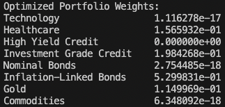
In percentages:

• Tech = 0%
• Healthcare = 15.7%
• HY Credit = 0%
• IG Credit = 19.8%
• Nominal Bonds = 0%
• Inflation-Linked Bonds = 53.0%
• Gold = 11.5%
• Commodities = 0%

So, basically, it likes some assets but doesn’t like others at all, effectively weighting them at zero.

In this particular algorithm, it picks the asset in the cluster it likes and down-weights the other to zero, then weights the “winner” of the cluster in relation to the other winners.

Asset Allocation – Hierarchical Risk Parity

FAQs – Hierarchical Risk Parity