Expected Asset Class Returns 5-10 Years Forward


This article was published on February 12, 2020
This article will look at estimates of what kind of financial returns can be expected out over the next 5 to 10 years. This will take into account the main asset classes – stocks (developed market, emerging), government bonds (developed market), credit, and alternative risk premia (private equity and real estate).
We will also look at the expected returns for cash, or essentially what short-term interest rates are likely to be.
While 2018 cheapened asset prices primarily due to the over-tightening of monetary policy by the Fed, 2019 made them more expensive again.
Forward returns fell from about 7 percent annualized for US equities toward the latter part of 2018 to just above 5 percent today. The forward returns on bonds also fell back to below the rate of inflation, meaning real returns are negative. This, in turn, brought up the price of gold, which tends to do well when real (i.e., inflation-adjusted) rates decline. Many forms of precious metals, particularly gold, given its use as a reserve currency, are used as currency hedges when real rates become unacceptably low.
With stocks at 5.2 percent forward returns and bonds at 1.6 percent (using the US 10-year), this puts the forward return for the traditional 60/40 portfolio at about 3.8 percent. Since 1900, the 60/40 allocation has averaged around 5 percent.
The 60/40 portfolio is anything but a balanced portfolio given stocks are more volatile than bonds. In reality, it’s more like 88/12 in terms of the risk decomposition. It is nonetheless a common benchmark. Portfolio construction is mostly beyond the scope of this article, though we address the subject in more detail in others.
What will the markets do over the intermediate term?
At the beginning of the year, projected forward asset returns look like the following:
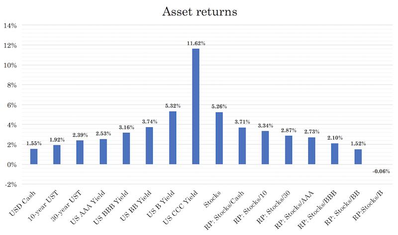
USD cash yields about 1.5 percent (3-month Treasury bills are taken as cash), while government bonds further out the duration curve don’t yield much more. Stocks are projected to yield just over 5 percent long-term.
AQR, which does their own projections, came out with the following in terms of their projections over the next 5- and 10-year periods. They compare estimates with January 2019 and January 2020. These are expressed in real terms. In other words, they are adjusted for inflation.
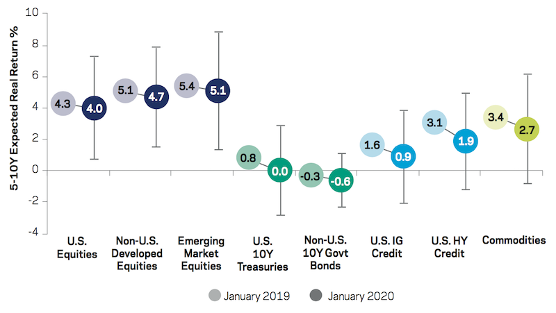
(Source: AQR. Estimates as of December 31, 2019)
Because of 2019’s returns pulling down forward returns, they expect US equities at 4.0 percent long-term, developed market equities (excluding US markets) at 4.7 percent, and emerging market equities at 5.1 percent.
US Treasuries are expected to deliver roughly nothing and negative returns for developed market sovereign debt. It’s hard to gain any return from bonds directly. In the US, their yields are very close to zero and currently negative in real terms.
Yields are already negative throughout most of developed Europe. That means you lose if bond prices stay put and lose if yields go up. The only way you “win” is if interest rates continue to decrease.
There is also the diversification and capital preservation angle for private investors. Governments and commercial banks are normally price-insensitive buyers of sovereign debt and government-backed securities. Central banks are typically motivated to buy them to carry out monetary policy operations or as a source of foreign currency reserves. Commercial banks often buy them to comply with regulatory mandates.
Lower interest rates will make cash a little bit less attractive to get people to take more risk, but if that’s the route that central banks want to go they still won’t be able to squeeze much more out of the bond market. Savers will still want to save, and lenders and borrowers will still remain cautious with each other.
Lower cash rates won’t get investors and savers into the type of assets that will help finance spending. Once the bond yields are maxed out as a stimulus form, central banks will likely need to remove the bond market as a constraining force to achieve their objectives and more directly target spenders and savers. This could either mean something like “helicopter money” (or giving people cash directly) or it could mean better fiscal and monetary policy coordination.
They also have investment grade (IG) credit at just a 0.9 percent long-term real return. For taking on more risk, high yield (HY) gives 1.9 percent. Commodities are expected to come in at around 2.7 percent real long-term.
Commodities are not a popular asset class among the public because the popular perception is that they don’t yield anything or they don’t produce cash. Commodities can be thought of as alternative stores of wealth, a growth-sensitive asset class, and a mix of individual markets subject to their own supply and demand considerations.
They’re not the best investments over time. But they do well in a certain environment and are key to having a balanced portfolio. If they are positioned right in a portfolio, they can be both return-enhancing and risk-reducing. I also own gold, but consider it more of an alternative currency and wealth storehold and less of something that’s supply and demand is based on its consumptive utility like oil, copper, or agricultural commodities. For those who do hold commodities, they should not be overemphasized in a portfolio.
Estimating forward financial asset returns
Over intermediate time horizons – say, 5-10 years – the current pricing and yields of financial assets tend to be the most important inputs.
When going out multiple decades – for example, a retirement account setup for a 25-year-old individual – the impact of starting prices and yields is not as influential.
In general, the average investor should not try to time the market or make tactical bets. They’re probably going to do that poorly and lose money relative to having a strong strategic asset allocation mix that’s structured to assume that the future is unknowable. Most people’s portfolios are constructed toward being long equities in their home stock market. This means they’re fundamentally betting on growth being above expectation. Because of the heavy environment bias, even in ostensibly balanced portfolios like the 60/40, these will have terrible drawdowns that will take a long time to dig back out of.
Over shorter time horizons, returns are hard to predict on the basis of starting prices or starting yields. Predictability in returns is often a reflection of what’s going on in the world in a macroeconomic sense or for momentum related reasons. What is meant by “momentum”? Momentum typically refers to the process by which people extrapolate what happened in the very recent past and assume that it will continue even if conditions change that make that a poor assumption.
Projections made over a medium time horizon can help investors calibrate the types of returns they can expect and what the returns of various allocations can yield. They are not intended to be of use for trading or market timing purposes.
Moreover, because of the annualized volatility of equities, over a 10-year period, there is roughly a 50 percent probability that equity markets will under- or over-perform these estimates by 3 percent or more.
Returns expectations should not be thought of as exact pinpointed calculations – though it can be useful to present the data as mean expected returns for simplicity – but as distributions of expected outcomes.
For example, if we were to input our returns assumption on a variety of assets on the following allocation:
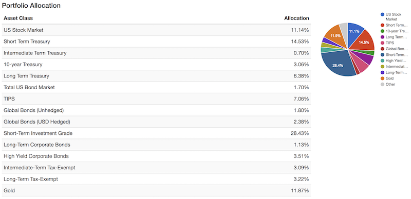
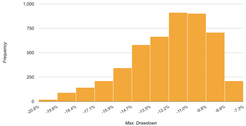
We would receive an expected returns range/distribution as such. This is on an unleveraged basis simulating out 75 years:
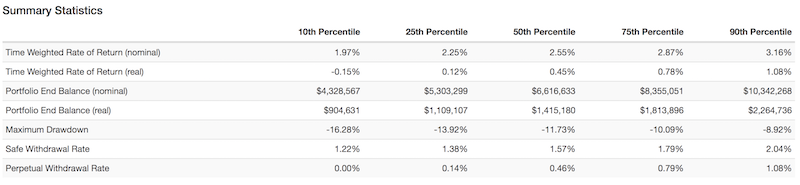
(Source: portfoliovisualizer.com)
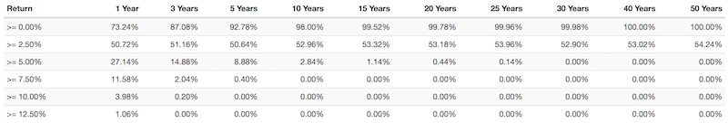
Annual return probabilities
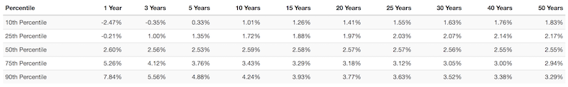
Returns of at least a certain threshold per year
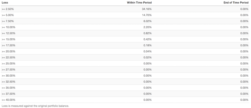
Loss probabilities
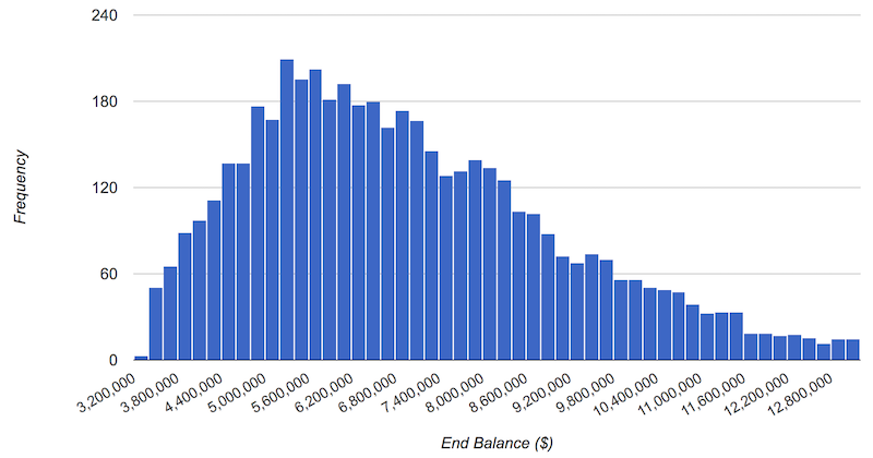
Portfolio End Balance Histogram (includes 95 percent of results)
Maximum Drawdown Histogram (includes 95 percent of results)
Forward returns as a function of the risk-free rate
Long-only investments have low expected returns due to their expensiveness. One way to tell that they’re expensive is by the fact that cash rates throughout the developed world are zero, nearly zero, or below zero. When rates get very low, there is limited ability to push them up higher because all assets are priced based on the present value of their future expected cash flows. When you can no longer lower this rate, you no longer have that tailwind to prices.
But even with low returns, the real equation you’re working with is cash against other financial assets. Borrowing at 0 percent to fund trades that’ll give you 5 percent is no different than borrowing at 5 percent (the average return of USD cash over the past half-century) and funding trades that yield you 10 percent. As one interpretation, investing is fundamentally about extracting risk premia from the market in the most efficient way possible.
If cash yields zero, to appropriately compensate you for a 2 percent return, that asset will likely have 6-10 percent volatility (to have a Sharpe ratio in the standard 0.2-0.3 range). If cash is zero, to keep that same type of ratio, you might expect equities to yield in the 3-4.5 percent range. This is very low relative to historical returns and carries high risk relative to return in absolute terms – a 4 percent return can be wiped out in a couple days, if not sooner – but is not terrible relative to cash.
Since AQR began estimating the forward intermediate returns of major asset classes in 2014, this is how these expectations have shifted over time.
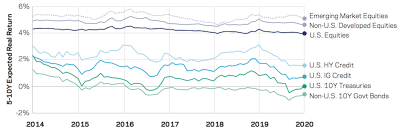
We can see emerging market equities offer the highest returns, while non-US developed market sovereign debt offers the least. The spread in real expected returns has trended pretty steadily between minus-1 percent and 6 percent.
That means if investors short the low yielding asset to fund the high yielding asset, they could expect to make a spread of 6-7 percent annually. This is risky because of the currency risk. Hedging currency risk would lower expected returns but not necessarily risk-adjusted returns.
Estimating returns by asset class
We’ll go through each asset class individually.
Equities
There are different ways to model the future returns on equities.
A simple way, for long-term considerations, is expected nominal growth rates. To keep expectations manageable, it’s important to remember that financial assets are simply claims on goods and services, and future expectations are already discounted in their prices.
A stock or bond, over the long-run, cannot increase faster than the goods and services output on which it’s a claim. At the index-wide level, this means gains in excess of growth are not sustainable long-term.
For more intermediate expectations, you can use discounted cash flow or the dividend discount model.
For the dividend discount model, you need the expected dividend yield, expected growth in earnings (or dividends), and expected change in valuation.
Namely, expected returns are equal to:
E[returns] = dividend yield + growth in earnings/dividends + change in valuation
Many will assume no changes in valuations. In today’s context, that means no reversion from the high valuations present in the current market. That effectively reduces the formula down to dividend yield and earnings per share (EPS) growth.
Earnings-based approach
On an earnings-based approach, using cyclically adjusted price-earnings (CAPE) over 10 years, this gives an inflation adjusted real earnings yield of 3.6 percent.
This is also known as the Adjusted Shiller E/P (earnings divided by price).
Multiplying this by 0.5 to reflect the long-run dividend payout ratio, or how much of this is paid out to shareholders, and adding to the earnings per share yield growth, this gives 3.3 percent (3.6 * 0.5 + 1.5)
In other words, under this formula, E[returns] = 0.5 * Adjusted Shiller E/P + growth in EPS
Payout-based approach
With a payout-based approach, the net total payout yield is the sum of the dividend yield and the net buyback yield. This is added to an earnings growth component (i.e., real GDP growth).
Therefore, payout-based expected return is equal to:
E[returns] = dividend yield + net buyback yield + E[EPS growth]
With a dividend yield of 1.8 percent, a net buyback yield of 0.2 percent and real aggregate earnings growth estimated at 2.6 percent, that gives a forward yield of 4.6 percent.
E[returns] = 1.8 + 0.2 + 2.6 = 4.6 percent
Combining the two
Taking a simple average of the two – 3.3 and 4.6 – this comes to about 4.0 percent.
From AQR’s 2019 estimates, this is 0.3 percent lower.
They do these estimates for all the main developed markets individually. The US has the lowest expected forward returns; emerging markets have the highest expected returns.
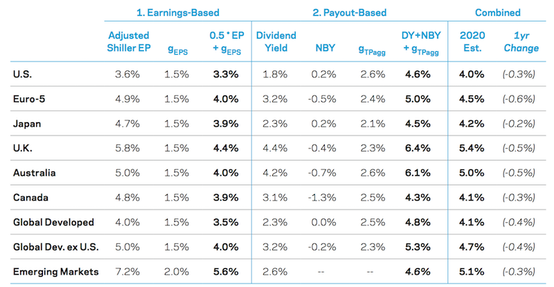
(Source: AQR, Consensus Economics and Bloomberg. Estimates and methodology subject to change and based on data as of December 31, 2019.)
Important notes on inflation and currency conversion
Local returns show only a partial reflection of expectations because the returns are shown in local currency.
To convert real returns to nominal returns, then expected inflation must be added.
To convert to real returns in excess of cash – i.e., your return beyond what your return would be if you didn’t take any risk – you need to subtract by an estimate of real expected cash return.
If you’re a foreign investor – e.g., US investor looking to buy Australian assets denominated in AUD – your expected return would need to be adjusted by correcting the expected cash rate differential plus the cross-currency basis (if hedging AUD assets back into USD), or the expected exchange rate return (if not hedging and keeping assets in AUD).
Generally speaking, those who decide to accept currency risk generally do so for the prospect of higher returns. However, for US investors who go into EUR and JPY asset markets and hedge back into USD, they will generally earn a higher return than taking on FX risk for reasons related to interest rate parity.
Interest rate parity states that currencies with lower interest rates are expected to trade at a higher exchange rate in the future. The market may anticipate inflection points in this relationship in the future – such as changes in one interest rate relative to another at a particular date due to the actions of central banks – that can cause the slope of the curve to change.
Examples
The implied forward exchange rate on the EUR/USD, one-year-forward, is 1.116 (at the time this is published, taking the midpoint). This is tradable as either a forward or swap. The spot rate is 1.091.
The implication is that, one year out, selling a EUR/USD 1-yr forward would net you about 2.3 percent in yield dividing those two figures (1.116 by 1.091). This is because you are effectively selling the EUR/USD exchange rate in one year’s time for a higher price than the current spot price.
If a US trader is buying a German bund at minus-50bps, the currency risk is hedged out by selling the EUR 1-yr forward or swap contract.
By doing so, this converts the bund proceeds into US dollars. Then we take the “yield” from the forward or swap, include the nominal yield of the bond (minus-0.50 percent) and come up with a dollar-hedged yield of about 1.8 percent.
In reality, it is not much different than investing in a US Treasury bond yielding 1.5-2.0 percent outside of the extra step of needing to hedge the currency. And there’s also some geographic diversification by branching into a different economy.
This process also works in reverse. From the European trader’s perspective, this currency hedge works in reverse. Unlike the US trader, who generates a positive yield on the hedge, the European trader pays it.
That means for the European trader, if he wants to buy a US Treasury bond at 1.6 percent and the cost of the hedge – to convert the proceeds of the Treasury bond back into EUR, his domestic currency – he has to pay 2.3 percent. The effective Treasury yield for the European trader is thus minus-0.70 percent. This is somewhat worse than the minus-0.50 percent yield.
With the currency conversion, that’s not much different than what the German bund yield despite the fact that the nominal yield differential, on the surface, tells you that US Treasury bonds are the better investment.
This is only true if yields are left unhedged. If the cross-currency basis is zero and the trader hedges, then the yield should be approximately the same between an equivalent duration US Treasury and German bund.
If the EUR-based trader wants to buy Treasuries but stays unhedged, he will be exposed to currency risk. He will effectively be long USD against the EUR. (This is how higher interest rates benefit a currency – they attract more capital inflows, holding all else equal.)
For the US trader, having his own currency that yields higher than other developed market currencies provides the chance to diversify among different markets while receiving a yield that’s comparable to US Treasuries.
For a US-based trader that wants to get involved in Switzerland, the 1-year forward rate on the USD/CHF is around 1.05 (taking the midpoint) against roughly 1.02 for the spot rate.
Swiss cash yields about minus-0.85 percent in CHF terms. Converting back to dollars (1.05 divided by 1.02, then adding the negative CHF yields), gives a FX-hedged yield of just over 2 percent. For those who are willing to take more duration risk, they can earn up to 2.5 percent on the long end of the curve.
Italian sovereign debt is some of the only EUR-denominated debt that still largely has a positive nominal and real yield due to its greater credit risk (because of material economic and political risks). The dollar-hedged equivalent yield on cash is about 2.05 percent, which would give the longest duration bonds nominal returns of more than 4 percent.
Government Bonds
Government bonds of reserve currency countries are largely assumed to be “risk free”. Namely, if you hold to maturity there is no material credit risk. These countries have control over their own money creation and these currencies have high foreign demand (for FX reserves, international payments and invoicing, and so on), which makes default highly unlikely.
The returns of government bonds over the intermediate term is strongly determined by their yields. Moreover, when the shape of the yield curve is positive or upward sloping, the return of a bond is somewhat higher than its yield.
A 10-year constant maturity US Treasury bond currently yields 1.6 percent. The rolling yield – or the additional capital gains from the rolldown as the bonds get closer to maturity – adds another 20bps of yield per year.
The rolling yields of six different countries, including global developed markets collectively and developed markets excluding the US (weighted by GDP), are included the diagram below. The data is from January 2020 when yields were slightly higher. The yields are converted to local real returns by subtracting estimates of longer-term inflation.
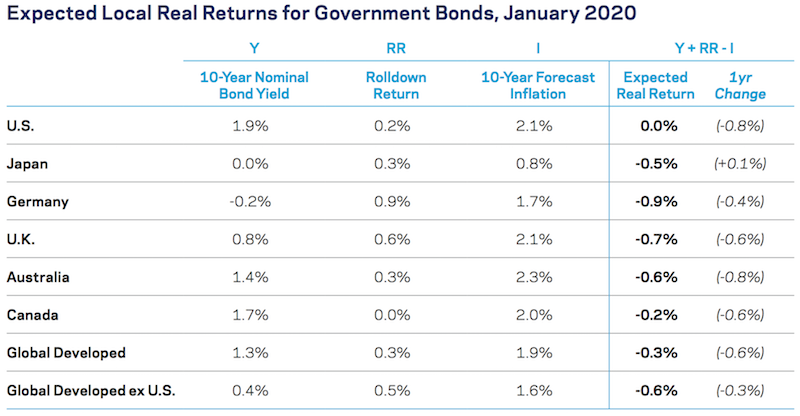
(Source: Bloomberg, Consensus Economics and AQR. Estimates as of December 31, 2019.)
Returns are uniformly zero to negative in real terms. Central banks have kept cash and bond yields low to keep interest rates low. This helps work off the high levels of debt relative to income and grapple with lower levels of productivity.
The capital gains from “curve rolldown” matter more in the short-run, as they cause day to day fluctuations (and more so for longer duration bonds). They matter less over longer periods of time.
These estimates also assume an unchanged yield curve, so fluctuations due to convexity and “volatility drag” are excluded. Volatility drag pertains to the reality that the more volatile your returns, the lower they tend to be under a random walk format.
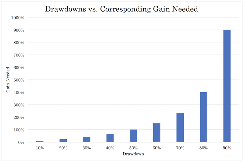
For example, if you were to oscillate between a 10 percent gain and 10 percent loss each day, you would not return zero, you would lose 1 percent per each two-day “cycle”: Amount left = starting amount * (1 + 0.1) * (1 – 0.1) = 0.99 of starting amount
Over 252 trading days per year, you would lose 72 percent of your money – 1 – .99^(252/2)
Because equal-percent gains do not compensate for their corresponding losses, this is one reason why drawdowns need to be avoided at all costs. It gets worse the larger the drawdown in a steepening, non-linear way.
Credit: US investment grade (IG), US high yield (HY), and Emerging Market Debt
Estimating the real returns for credit involves applying an assumed loss amount for both IG and HY returns from rating agency downgrades and default losses. There is no assumed change in the spread between government debt and corporate yields.
Essentially we take the ingredients from the returns in the respective government bonds markets and add a spread component:
Credit real yield = Government bond real yield + Rolldown yield + Credit spread
Credit is much more expensive in 2020 relative to 2019. In 2019, because Fed tightening had reached its peak, Treasury yields were higher and credit markets had baked in higher credit risk due to the increased default probabilities.
Expected real returns, credit, January 2020
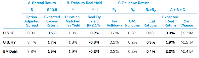
(Source: Barclays, Bloomberg, AQR. Estimates as of December 31, 2019. OAS and duration data is for Barclays U.S. Corporate Investment Grade (IG) Index, Barclays U.S. Corporate High Yield (HY) Index and Barclays Emerging USD Sovereign (EM Debt) Index. Index durations are 7.9 years, 3.1 years and 7.7 years, respectively.)
Commodities
Commodities, as physical non-cash producing entities, do not have clear yields associated with them.
They also tend to be even more volatile than equities, though they are less prone to valuation distortions due to narrative.
Predicting broad commodity returns over a 5-10 year time scale is difficult. Accordingly, over that timeframe, your expected returns can be reduced to a representative portfolio of commodity futures.
Since 1877, such a portfolio has earned 3.0 percent in excess of cash. It has also obtained a comparable return since 1951, taking a more truncated data set. Because the US inflation-adjusted cash return is now negative – 150bps minus inflation of around 200bps – this gives an expected real return of around 2.5 percent.
Alternatives
Value, long-only equity
Value looks more reasonably priced compared to growth. If diversified well and charging 1 percent of assets and no performance fee, this type of portfolio could return 50-100bps higher than the market with a tracking error (i.e., standard deviation of excess returns) of around 300bps.
Multi-strategy equity
Beyond value, one that’s better diversified among various factors, such as value, defensive, dividend, and growth, may achieve an excess return of ~100bps over the market after fees (charging 1 percent and no performance fee). This comes with a similar tracking error of around 300bps.
Diversification across multiple asset classes
Beyond equities, a portfolio such as risk parity that is well diversified across many assets classes (equities, fixed income, commodities, foreign currencies, including both domestic and internal exposure) can achieve a Sharpe ratio of more than 0.5, compared with 0.2-0.3 by focusing on just one asset class.
Learning to diversify well is the most valuable thing you can do to improve your return per unit of risk without having to pick what assets are going to do well or try to time the market and get in or out when things are good or bad.
If pegged to an equity-like volatility – i.e., around 15 percent – then your excess returns over cash should be about 7-8 percent annualized. If targeting 10 percent volatility (about two-third the volatility of equities), then excess returns over cash should approximate 5 percent.
Getting these types of returns requires careful portfolio design and implementation and portfolio management. This mean controlling trading costs, shorting costs, financing costs, and maintaining generally disciplined trade activity. If not done successfully, then such portfolios can have much lower expected returns.
What about valuation differences on long-run returns?
Growth and momentum are expensive, as is defensive (e.g., utilities). Value is relatively cheap, and value is disproportionately founds in small and mid cap stocks, as opposed to large cap where growth dominates.
With that said, the relationship between valuation and valuation spreads (i.e., growth vs. value) and future returns are weak. Timing when to buy “cheap” assets and when to sell (or short-sell) “expensive” assets is difficult to do and difficult to outperform a strategic multi-asset or multi-style portfolio over a longer period of time.
Private Equity and Real Estate
Assets that are inherently illiquid and aren’t consistently marked to market are more difficult to model than liquid, public-market securities. Data is often speculative and non-transparent.
Private equity (US)
Because of data limitations, private equity data requires some simplifying assumptions.
Fees are a material component of the returns in illiquid asset classes. Naturally, to get at returns, we need to present these outputs as net of fees.
Unleveraged expected returns are equal to the sum of the unlevered payout yield and the inflation-adjusted growth rate in earnings per share.
The leveraged return is then a function of multiplying unleveraged expected returns by the turns of leverage used minus the cost of the debt. From there, add in any expected multiple expansion and subtract out any fees taken by the manager.
With an estimated unlevered payout yield of 2.0 percent and real EPS growth rate of 3.0 percent, that gives an unlevered real return estimate of 5.0 percent.
If the debt to equity ratio is 86 percent (in other words, the deals are about 54 percent equity and 46 percent debt, based on 1 divided by 1.86) and the effective cost of debt is 1.6 percent, this gives a return of:
5 percent * 1.86 – 0.86 * 1.6 percent = 8.1 percent
Subtracting out fees of 5 percent, this gives a net return of 3.1 percent. This expected return is down 80bps from 2019.
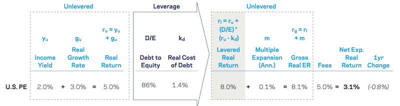
(Source: AQR, Pitchbook, Bloomberg, CEM Benchmarking. Estimates as of September 30, 2019 and are subject to change. Historical averages cover the period January 1993 to September 2018. These inputs are log returns and should be converted to simple returns before leverage is applied, then converted back to log returns. Because of its small impact, this step was omitted for simplicity.)
A yield-based return gives 5.1 percent net of fees (nominal), or 3.1 percent real.
Using a public proxy, assuming zero alpha (i.e., net value added) and making basic leverage and size adjustments, this gives a higher estimate of 7.5 percent (nominal), or 5.5 percent real.
Using the average of the two approaches, these give a real estimate of 4.3 percent. This is slightly above the US public equity estimate of 4.0 percent.
Private US real estate
The returns for individual real estate funds can vary significantly from the industry average, as can be said for private equity.
We can use indices from the National Council of Real Estate Investment Fiduciaries (NCREIF) to estimate expected returns for unlevered direct real estate investing.
Using the same dividend discount model approach for estimating equities returns, we can use the sum of the payout yield and the expected long-term growth rate. This shows an expected real return of about 3 percent for unleveraged real estate.
This is the sum of net operating income, capital expenditure (an outlay, so therefore subtracted), and real growth.
If net operating income is 4.7 percent, capital expenditure is 1.6 percent, and real growth is zero, that gives the approximate 3 percent unleveraged return.
Expected Real Returns for U.S. Private Real Estate
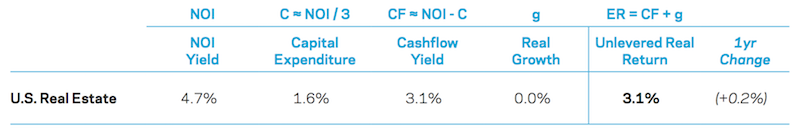
(Source: AQR, NCREIF Webinar Q3 2019. Estimates as of September 30, 2019 and subject to change.)
The Estimated Return on Cash
Asset allocation decisions are typically made based on expected returns “excess of cash”.
In terms of expected returns, you have three basic building blocks:
– Cash – also known as the risk-free rate as it’s the equivalent to short-term government “bills” (like 3-month US Treasuries or UK gilts)
– Beta – the returns associated with investing in an individual asset class (stocks, bonds)
– Alpha – deviating from the betas
When the returns on betas become unattractive – e.g., a yield curve inversion, which makes cash rates relative to longer-term lending rates – more people opt for cash.
But cash will underperform other financial assets over time. If it doesn’t, then capitalist economies won’t work well for any elongated period and central banks will have great incentives to get money and credit creation going again. People who have good uses for cash will borrow it to create something of higher value (i.e., beyond the interest returned on the cash).
Cash isn’t a material source of return in developed markets. The nominal return is zero or negative through Japan and developed Europe and is negative in real terms in the US as well.
The expected cash rate, either real or nominal, is an important input in asset allocation decisions. Moreover, it is a big part of the equation in determining where to invest capital.
People will look at the forward returns of stocks somewhere around 5 percent annualized and think the return is poor. It is poor in absolute terms and relative to their risks.
However, if you can borrow at zero percent, your return is five percent, that’s no different than borrowing at 5 percent and investing at 10 percent.
Whether these returns are expressed as nominal or real, it doesn’t matter so long as they are congruent (and not real for one variable and nominal for another).
Investing is really about extracting a spread. What’s your return on cash and/or your return on what you’re borrowing, and what can you earn in excess of that?
To determine future cash rates, we can use the current long-term government bond as a proxy. A long-term bond is the function of the market’s expectations for where short-term yields are likely to be plus a term premium, which is not directly observable and varies over time. (The term premium is theoretically what your return would be if you invested in short-term government bonds and rolled them continuously to the chosen maturity.)
In the graph below, the expected returns on cash from both short-term and long-term bonds pegs it at just under 2 percent over the long-run.
US Bond and Bill Yields, Cash Forecast and Subsequent Cash Rate 1960-2020
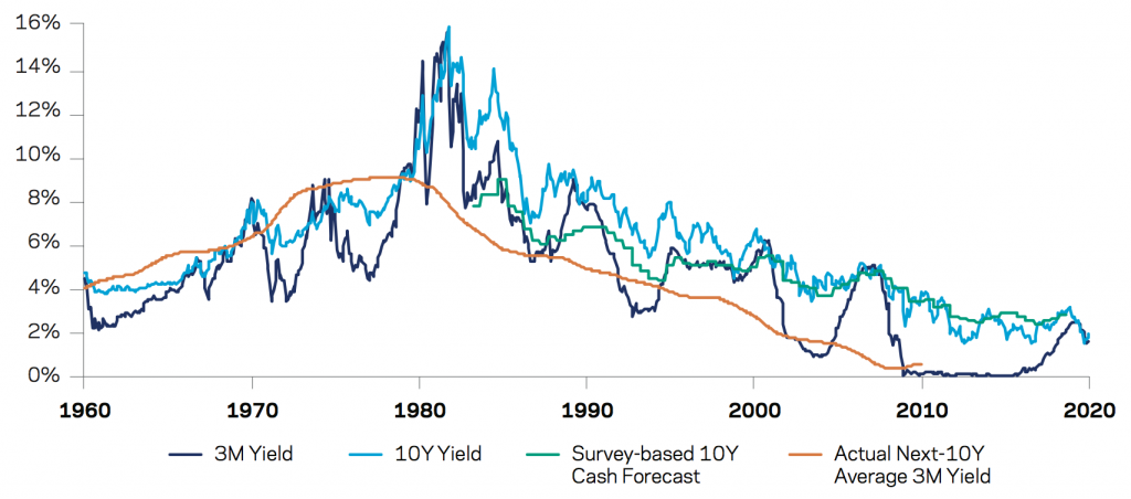
(Source: Global Financial Data, Blue Chip Economic Indicators and AQR.)
The short-term Treasury bill consistently underestimated future cash yields in the 1960s and 1970s and overestimated them in the 1980s on forward.
US-specific survey results began in 1983 and have consistently underestimated cash rates out one decade, and by nearly 4 percent.
Modeling future cash rates as a weighted average, we can integrate signals from various parts of the yield curve, such as both the 3-month yield, 2-year yield, 10-year yield, and 30-year yield. Putting an equal weight in each would derive a future US cash yield expectation of 1.65 percent.
If one were to put two-thirds of the weight on the 10-year, one-third on the 3-month yield and subtract the 10-year inflation forecast to derive a real cash rate, we get the following for the main six developed countries (US, Japan, Germany, UK, Australia, and Canada).
Expected Local Real Returns for Cash, January 2020
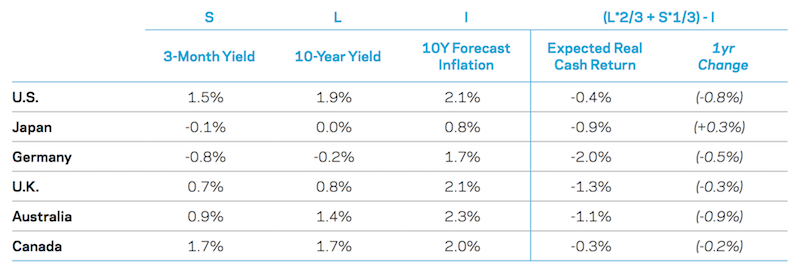
(Source: Bloomberg, Consensus Economics and AQR. Estimates as of December 31, 2019.)
Conclusion
When you look at the returns on cash and bonds, you see that they are closer to being funding vehicles than actual quality investments.
That leaves you with equities and alternative/equity-like investments such as real estate, private equity, and private lending. And these are only giving you 3 to 6 percent in excess of cash.
Because most traders and investors extrapolate the past and assume that past returns will be indicative of future returns, they are likely to be sorely disappointed. Return objectives are not likely to be met with such an unappealing slate of low-yielding assets.
This has implications for unfunded pension obligations and younger investors who are likely to struggle to build wealth over the long-term. Expected contributions to worker pensions will almost surely need to go up while expected payouts will need to be lower.
Many traders will also take the risk of leveraging up in a low forward-return environment to achieve their desired returns on equity. This compounds the problem because more leverage in portfolios at large will exacerbate moves back in the other direction when the time comes.
Forward low returns should not be taken an implicit “recommendation” to be more aggressive in one’s tactical asset allocation.
Over the short- and medium-term the returns of asset classes are very difficult to pin down within any degree of precision, though we can give reasonable estimates. A 30 percent annual swing in the equities market either way is fully within the range of expectations. Moreover, in low interest rate environments, the duration of assets lengthens, which makes their prices more sensitive to movements in interest rates.
Having a portfolio that is well-diversified across many asset classes and risk premia (fixed income, equities, real estate, private investments) is likely to deliver the best results over the long-term.