Estimation Theory in Finance

Estimation theory is a branch of statistics that helps to infer values of unknown parameters within financial models.

This process involves using statistical methods to estimate these parameters based on observed data. 

Estimation theory can be used in asset pricing, risk management, portfolio construction, and various other areas of quantitative finance.

Key Takeaways – Estimation Theory

• Fundamental Concept of Unbiased Estimators:
  • Estimation theory emphasizes the importance of using unbiased estimators in statistical analysis.
  • Ensures that the expected value of these estimators matches the true parameter values.
  • Helps provide accurate and reliable estimates over many samples.
• Efficiency and Consistency:
  • The theory prioritizes efficiency.
    • Means that among unbiased estimators, those with the lowest variance are preferred.
  • Consistency is also important.
    • Ensures that as sample size increases, the estimator converges in probability to the true parameter value.
• Role of Maximum Likelihood Estimation (MLE):
  • MLE is a central technique in estimation theory.
    • Provides a method for estimating the parameters of a statistical model.
  • It selects the parameter values that maximize the likelihood function, often leading to more accurate and efficient estimators in many practical applications.
• Examples
  • We use examples of linear regression and Monte Carlo simulations below.

Core Principles of Estimation Theory

Understanding Statistical Estimators

A statistical estimator is an algorithm or a formula that aids in deducing the unknown parameters of a given population from observed data. 

In finance, these estimators help in making inferences about market returns, volatility, correlations, and other financial metrics.

Types of Estimators

Two primary types of estimators are widely used:

• point estimators
• interval estimators

Point estimators provide a single value estimate of a population parameter, like the mean return of a stock. 

Interval estimators, on the other hand, offer a range within which the parameter is expected to lie, accounting for uncertainty and variability in the data.

Application of Estimation Theory in Finance

Asset Pricing Models

Estimation theory is instrumental in developing and refining asset pricing models like the Capital Asset Pricing Model (CAPM) and the Arbitrage Pricing Theory (APT). 

It helps in estimating the parameters like beta in CAPM, which measures a stock’s volatility relative to the market.

Risk Management

In risk management, estimation theory is used to quantify risk metrics such as Value at Risk (VaR) and Conditional Value at Risk (CVaR). 

Estimators help in assessing the likelihood of financial losses under normal and extreme market conditions.

Portfolio Optimization

Portfolio optimization relies heavily on estimation theory to determine the optimal allocation of assets. 

Estimators are used to gauge expected returns, variances, and covariances of asset returns, important for constructing efficient portfolios.

Challenges in Estimation Theory

Data Quality and Availability

The accuracy of estimators heavily depends on the quality and quantity of available data. 

In financial markets, this includes dealing with noisy, non-stationary, and sometimes incomplete data sets.

Model Assumptions

Many financial models based on estimation theory operate under specific assumptions like normality of returns or linear relationships between variables. 

Violations of these assumptions can lead to biased or inconsistent estimates.

Many returns are fat-tailed or don’t neatly fit any parametric approach.

Overfitting and Underfitting

There is a balance in model complexity. 

• Overfitting involves creating models that are too complex and fit the noise in the data.
• Underfitting models are too simplistic to capture the underlying dynamics of financial markets.

Future of Estimation Theory in Finance

Advancements in computational power and machine learning algorithms are expanding the horizons of estimation theory in finance. 

Techniques like Bayesian estimation, Monte Carlo simulations, and machine learning models are increasingly being adopted for financial data and provide more robust and accurate estimations. 

The future of estimation in finance is geared towards more adaptive, data-driven models capable of handling the various nuances in financial markets (e.g., machine learning).

Estimation Theory – Python Code (Monte Carlo Simulation)

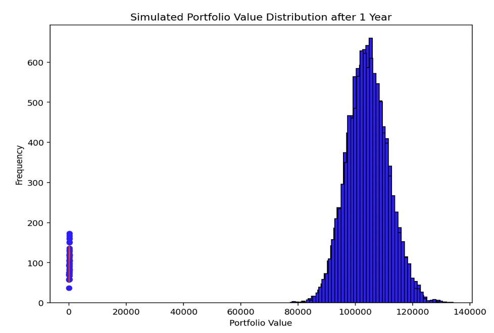
The Monte Carlo simulation, as shown in the Python code, forward tests the distribution of a specific portfolio over one year.

The portfolio consists of Stocks, Bonds, Cash, and Gold, with predetermined allocations and their respective expected returns and volatilities.

Key aspects of this simulation include:

Portfolio Composition

The portfolio is composed of four assets:

• 35% Stocks
• 40% Bonds
• 10% Cash
• 15% Gold

Each asset class has its own expected forward return and annualized volatility (except for Cash, which has zero volatility).

• Stocks: 6% forward return, 15% annualized volatility using standard deviation
• Bonds: 3.5% forward return, 10% annualized volatility using standard deviation
• Cash: 3% forward return, 0% annualized volatility using standard deviation
• Gold: 3% forward return, 15% annualized volatility using standard deviation

Simulation Parameters

The simulation runs 10,000 iterations to generate a wide range of possible outcomes.

The time horizon is set to one year, and the initial investment is $100,000.

Simulation Process

For each iteration, the final portfolio value is calculated by applying the return and volatility of each asset class, considering their respective allocations.

The assumption that the assets are not correlated is maintained throughout the simulation.

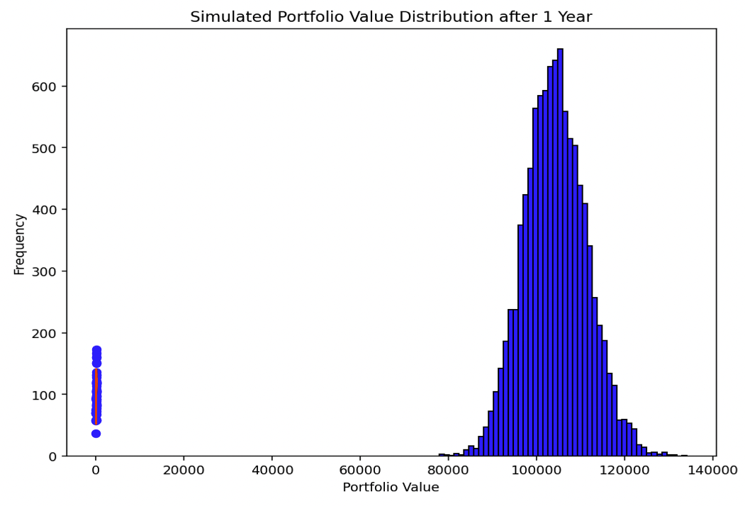
Results Visualization

The histogram displays the distribution of the final portfolio values across all simulations.

This distribution provides insights into the range and likelihood of various portfolio outcomes after one year, considering the specific asset allocation and market conditions defined for each asset class.

This simulation helps in understanding the potential risk and return profile of the given portfolio.

The distribution can also be repeated if you want another look at it.

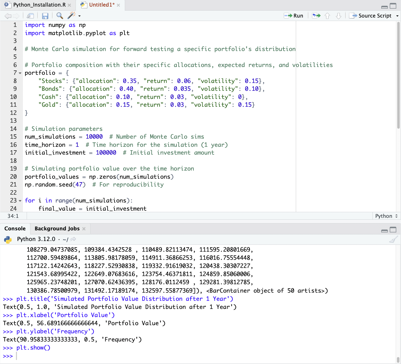
Here’s the code:

import numpy as np
import matplotlib.pyplot as plt

# Monte Carlo simulation for forward testing a specific portfolio's distribution

# Portfolio composition with their specific allocations, expected returns, and volatilities
portfolio = {
"Stocks": {"allocation": 0.35, "return": 0.06, "volatility": 0.15},
"Bonds": {"allocation": 0.40, "return": 0.035, "volatility": 0.10},
"Cash": {"allocation": 0.10, "return": 0.03, "volatility": 0},
"Gold": {"allocation": 0.15, "return": 0.03, "volatility": 0.15}
}

# Simulation parameters
num_simulations = 10000 # Number of Monte Carlo simulations
time_horizon = 1 # Time horizon for the simulation (1 year)
initial_investment = 100000 # Initial investment amount

# Simulating portfolio value over the time horizon
portfolio_values = np.zeros(num_simulations)
np.random.seed(0) # For reproducibility

for i in range(num_simulations):
final_value = initial_investment

# Calculating portfolio value at the end of time horizon for each asset
for asset, info in portfolio.items():
annual_return = info["return"]
annual_volatility = info["volatility"]
random_return = np.random.normal(annual_return, annual_volatility)
final_value += final_value * info["allocation"] * random_return

portfolio_values[i] = final_value

# Plotting the distribution of portfolio values
plt.hist(portfolio_values, bins=50, color='blue', edgecolor='black')
plt.title('Simulated Portfolio Value Distribution after 1 Year')
plt.xlabel('Portfolio Value')
plt.ylabel('Frequency')
plt.show()

If using this code, be sure to indent where appropriate given indentation is important in Python:

Estimation Theory – Python Code (Linear Regression)

In this example, linear regression is applied to understand the relationship between a company’s earnings and its stock price:

Synthetic Data Generation

Synthetic data for earnings (in million dollars) and stock prices of 50 companies is created.

The earnings are normally distributed, and stock prices are modeled to be related to these earnings.

Linear Regression Model

The LinearRegression model is fitted to this data, with earnings as the independent variable and stock prices as the dependent variable.

Related: Stock Prices and Linear Regression

Relationship Estimation

The coefficient obtained from the model indicates the relationship between earnings and stock prices.

In this context, it represents how much the stock price is expected to increase for every million dollar increase in earnings.

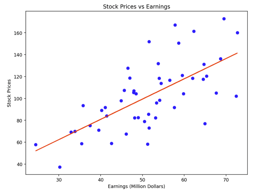
Visualization

A scatter plot is shown with earnings on the x-axis and stock prices on the y-axis, along with the regression line.

This plot visualizes the correlation between a company’s earnings and its stock price.

This analysis highlights how estimation theory, through linear regression, can be used in finance to understand and quantify relationships between different financial metrics.

import numpy as np
import pandas as pd
import matplotlib.pyplot as plt
from sklearn.linear_model import LinearRegression

# Generating synthetic data for stock prices and earnings
np.random.seed(0)
companies = 50
earnings = np.random.normal(50, 10, companies) # Earnings in million dollars
stock_prices = earnings * np.random.normal(2, 0.5, companies) # Stock price related to earnings

# Creating a DataFrame
data = pd.DataFrame({'Earnings': earnings, 'Stock_Prices': stock_prices})

# Applying Linear Regression
model = LinearRegression()
model.fit(data[['Earnings']], data['Stock_Prices'])

# Estimating the relationship
relationship = model.coef_[0]

# Plotting
plt.scatter(data['Earnings'], data['Stock_Prices'], color='blue')
plt.plot(data['Earnings'], model.predict(data[['Earnings']]), color='red')
plt.title('Stock Prices vs Earnings')
plt.xlabel('Earnings (Million Dollars)')
plt.ylabel('Stock Prices')
plt.show()

relationship

FAQs – Estimation Theory

What is Estimation Theory in Finance?

Estimation theory in finance involves using statistical methods to determine unknown parameters within financial models based on observed data.

It helps in making educated guesses about important financial metrics, like stock returns or market volatility.

This theory is important in areas like asset pricing, risk management, and portfolio optimization, where accurate estimates guide investment decisions and risk assessments.

How Does Estimation Theory Work in Asset Pricing Models?

Estimation theory in asset pricing models involves calculating parameters like beta in the Capital Asset Pricing Model (CAPM), which indicates a stock’s risk relative to the market.

It helps in estimating expected returns based on historical data, considering factors like market risk premium and the risk-free rate.

Estimation theory enables traders, investors, and analysts to make informed decisions based on historical market behaviors and statistical analyses.

How Does Estimation Theory Contribute to Risk Management in Finance?

In risk management, estimation theory is key to quantifying risk metrics such as Value at Risk (VaR) and Conditional Value at Risk (CVaR).

These metrics estimate potential losses in a portfolio, considering historical market trends and volatility.

Estimation theory helps in forecasting the likelihood and magnitude of losses under various market conditions.

This helps risk managers develop strategies to mitigate potential financial risks and to understand the risk-return trade-off in their choices.

What Are the Most Common Statistical Methods Used in Financial Estimation?

Common statistical methods in financial estimation include regression analysis, time-series analysis, and Monte Carlo simulations.

Regression analysis is used to understand relationships between financial variables.

Time-series analysis helps in forecasting future market trends based on past data.

Monte Carlo simulations are used for assessing the impact of risk and uncertainty in financial models by simulating a wide range of possible outcomes (and is non-parametric in nature).

These methods provide a framework for analyzing complex financial data and making informed estimates.

How Does Estimation Theory Assist in Portfolio Optimization?

Estimation theory assists in portfolio optimization by estimating expected returns, variances, and covariances of asset returns.

These estimations are fundamental in constructing efficient portfolios that aim to maximize returns for a given level of risk.

By using historical data and statistical models, estimation theory guides the allocation of assets in a portfolio, balancing the trade-off between risk and return, and helps in achieving diversification to reduce overall portfolio risk.

What Are the Limitations and Challenges of Using Estimation Theory in Financial Analysis?

The limitations and challenges of using estimation theory in financial analysis include data quality issues, model assumptions, and the risk of overfitting or underfitting.

Financial data can be noisy and non-stationary, which might lead to inaccurate estimates.

Assumptions like normality of returns or linear relationships may not always hold true, leading to biased estimates.

Overfitting, where models capture noise instead of underlying trends, and underfitting, where models oversimplify the data, are challenges.

These limitations necessitate careful model selection, validation, and continuous adaptation to make sure they fit existing (and future) market conditions.