How Accurately Can Stock Prices Be Estimated Through Linear Regression?

It is one of the most common statistical methods that individuals use to analyze data on a vast assortment of data.

Can this be accurately be done with respect to estimating stock prices as a means of fundamental analysis?

The short answer is that it potentially can be one of the many ways to analyze what impacts prices if our data set is divided appropriately, either by economy, sector, and so forth.

The dividend discount model (DDM) is a valuation model in finance that allows us to help estimate stock prices and is applicable to all stocks that pay dividends.

In order to apply linear regression, we need to understand if our data is normal or not, meaning whether it fits the normal distribution. This is inherent in the assumption of being able to apply linear regression to a set of data in the first place.

To determine our answer, we can run a Monte Carlo simulation on the Gordon Growth Model that is built into the mathematical infrastructure of the DDM model. It can also help us discern some relationships between stock price and other variables first.

We can apply the following equation, which, within the DDM model, allows us the means to determine how the present value of future dividends in order to determine proper stock price estimation:

P = D / (r – g)

Where:

P = Price of stock
D = Value of next year’s dividends
r = Cost of equity in the stable growth phase of the company
g = Growth rate in stable growth phase

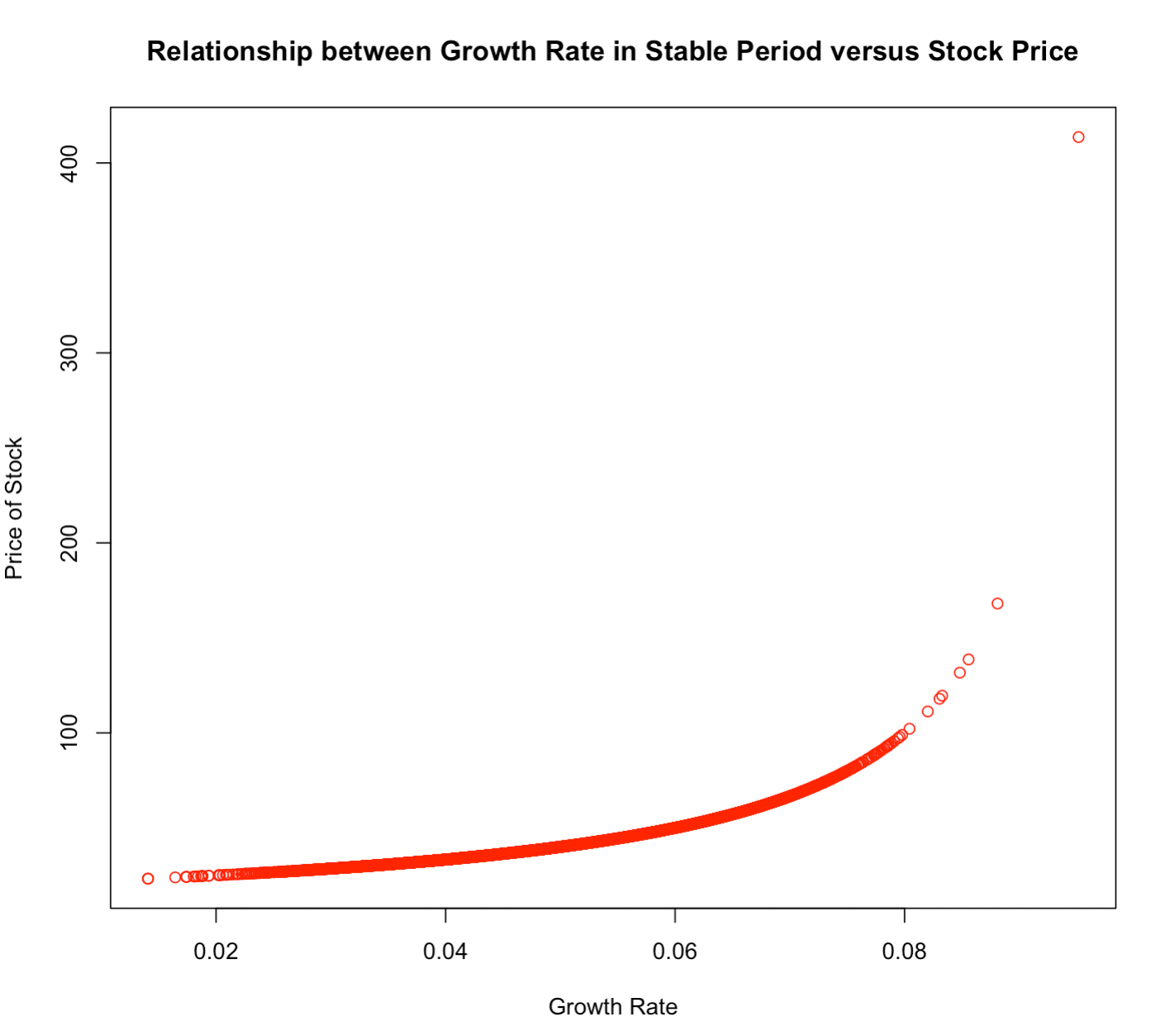
Once the growth rate approaches the cost of equity, that denominator becomes continuously smaller to the point where the stock price increases in steepening, non-linear fashion.

Doing a basic Monte Carlo simulation in R software, we can graphically observe things directly.

Let’s say a company will pay out dividends of $2.00 per share next year, cost of equity is 10% (the return needed to incentivize investors to purchase shares of the company), and the growth rate will be randomly generated 10,000 times with a mean of 5% and a standard deviation of 1%, which would be a fairly standard nominal growth rate for the economy as a whole.

We will paste the code in various spots of the article (gray boxes) should you wish to try these R simulations yourself.

D <- 2

r <- .1

g <- rnorm(10000,.05,.01)

P <- D / (r - g)

plot(g, P, main="Relationship between Growth Rate in Stable Period versus Stock Price",
xlab="Growth Rate", ylab="Price of Stock", col="red")

From the graph we can observe a clear exponential relationship between the factors of growth rate in the stable period and stock price:

We can also perform a simulation of the stock price of multiple companies by simulating both the cost of equity and stable period growth rate.

If we simulate the cost of equity with a mean of 10% and a standard deviation of 1% (these figures are arbitrarily chosen, but will demonstrate the relationship) and vary the growth rate similarly (mean = 5%, standard deviation = 1%), we have a figure that resembles this:

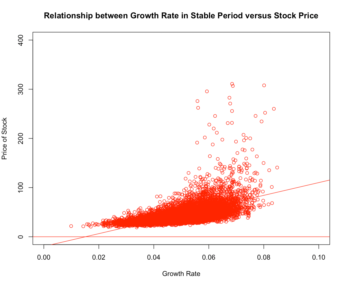
We have a few outliers, with some companies with inflated estimated stock prices due to the smallness of the denominator from a low cost of equity and/or high growth rate (rather than genuine high performers).

D <- 2

r <- rnorm(10000,.1,.01)

g <- rnorm(10000,.05,.01)

P <- D / (r - g)

lm (P ~ g)

plot(g,P, main="Relationship between Growth Rate in Stable Period versus Stock Price",
xlab="Growth Rate", ylab="Price of Stock", col="red",
xlim=c(0,.1),ylim=c(0,400))

abline(lm(P~g), col="red")

abline(h=0, col="red")

This simulates the stock price of 10,000 different companies under these same, relatively homogenous economic parameter inputs. A line of best fit shows a positive relationship naturally, and with more variety in stock price as growth rate increases.

We can test for normality in the data using quantile regression, to determine whether stock price’s relationship with growth rate and cost of equity can be modeled linearly.

For stock price versus growth rate:

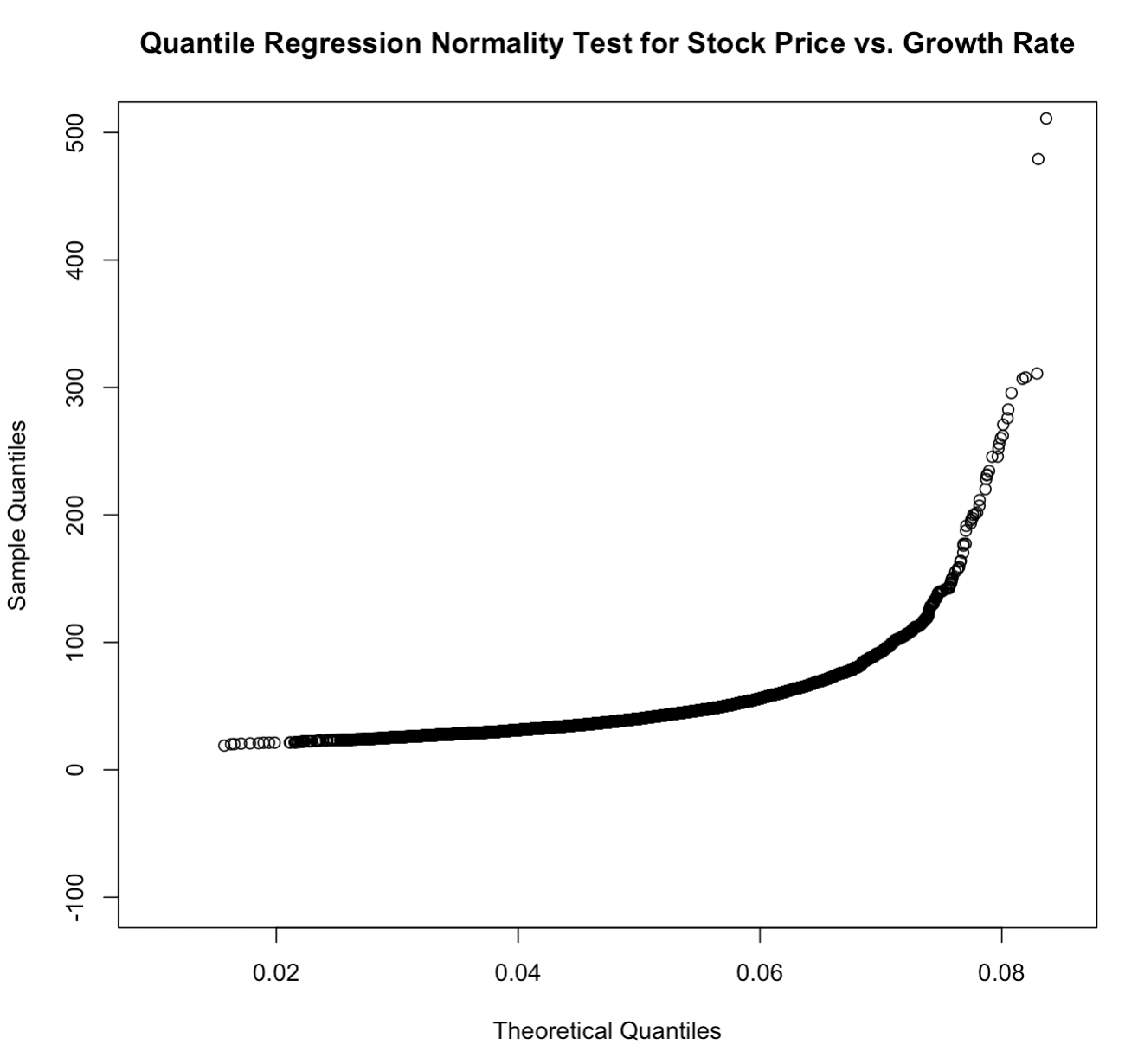
 qqplot(g, P,xlab = "Theoretical Quantiles", ylab = "Sample Quantiles",
       main="Quantile Regression Normality Test for Stock Price vs. Growth Rate",
       ylim=c(-100,500))

For stock price versus cost of equity:

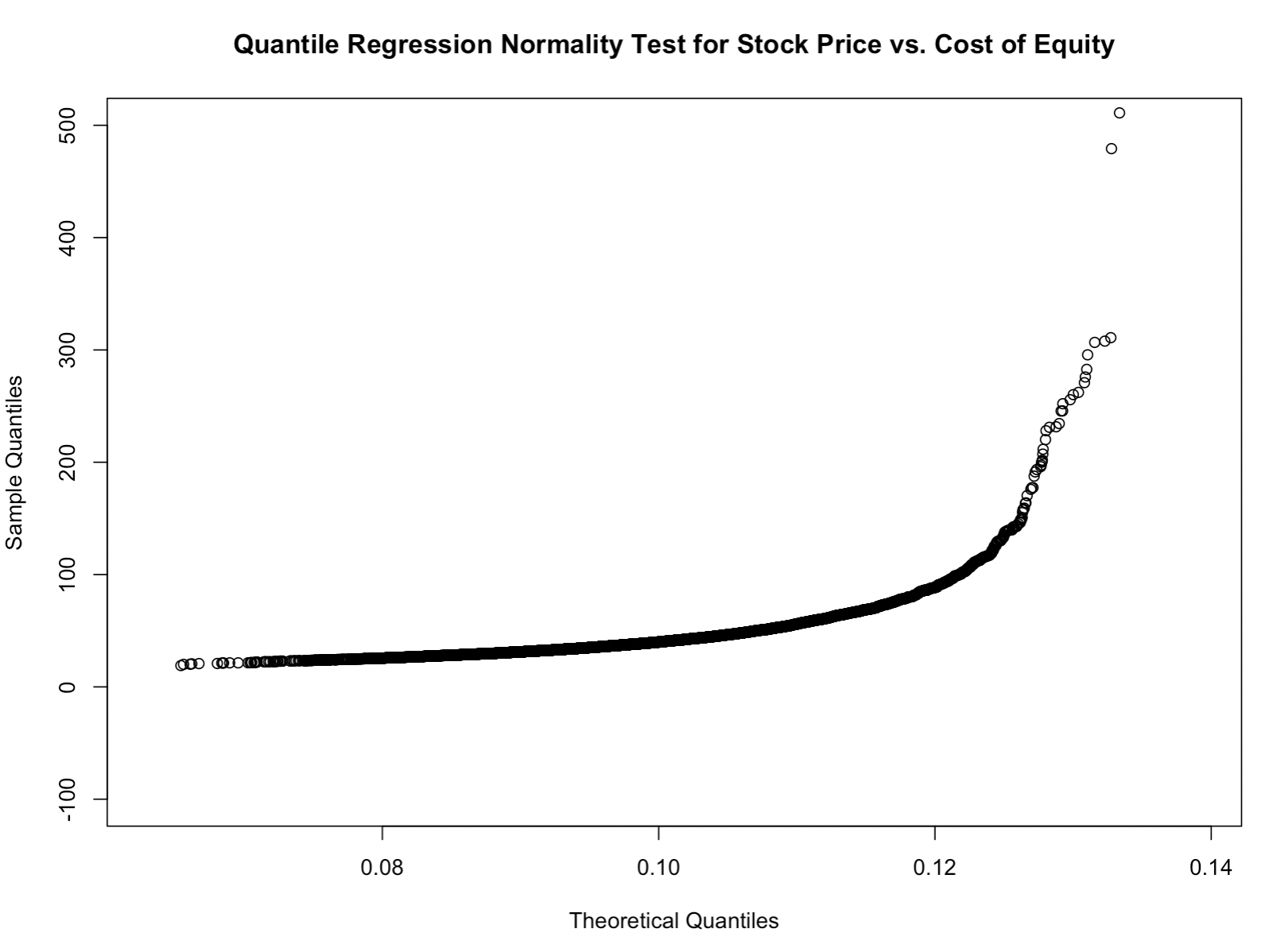
 qqplot(r, P,xlab = "Theoretical Quantiles", ylab = "Sample Quantiles",
       main="Quantile Regression Normality Test for Stock Price vs. Cost of Equity",
       ylim=c(-100,500))

Being the data do not fit a straight line, we know that the data do not pass a normality test as it relates to growth rate and cost of equity as they pertain to stock valuation at outlier-type values.

If we develop an actual linear model, for instance, stock price regressed on cost of equity and growth rate, we observe the maximum level of statistical significance for each independent variable.

And also, both variables are of the correct sign – negative for cost of equity and positive for growth rate.

This means a lower cost of equity will tend to lower stock price (true) and a higher growth rate of the firm will tend to raise stock price (also true).

model1 <- lm(P ~ g + r)

summary(model1)

It also reasonably passes our quantile regression test for normality, given the straight line shape:

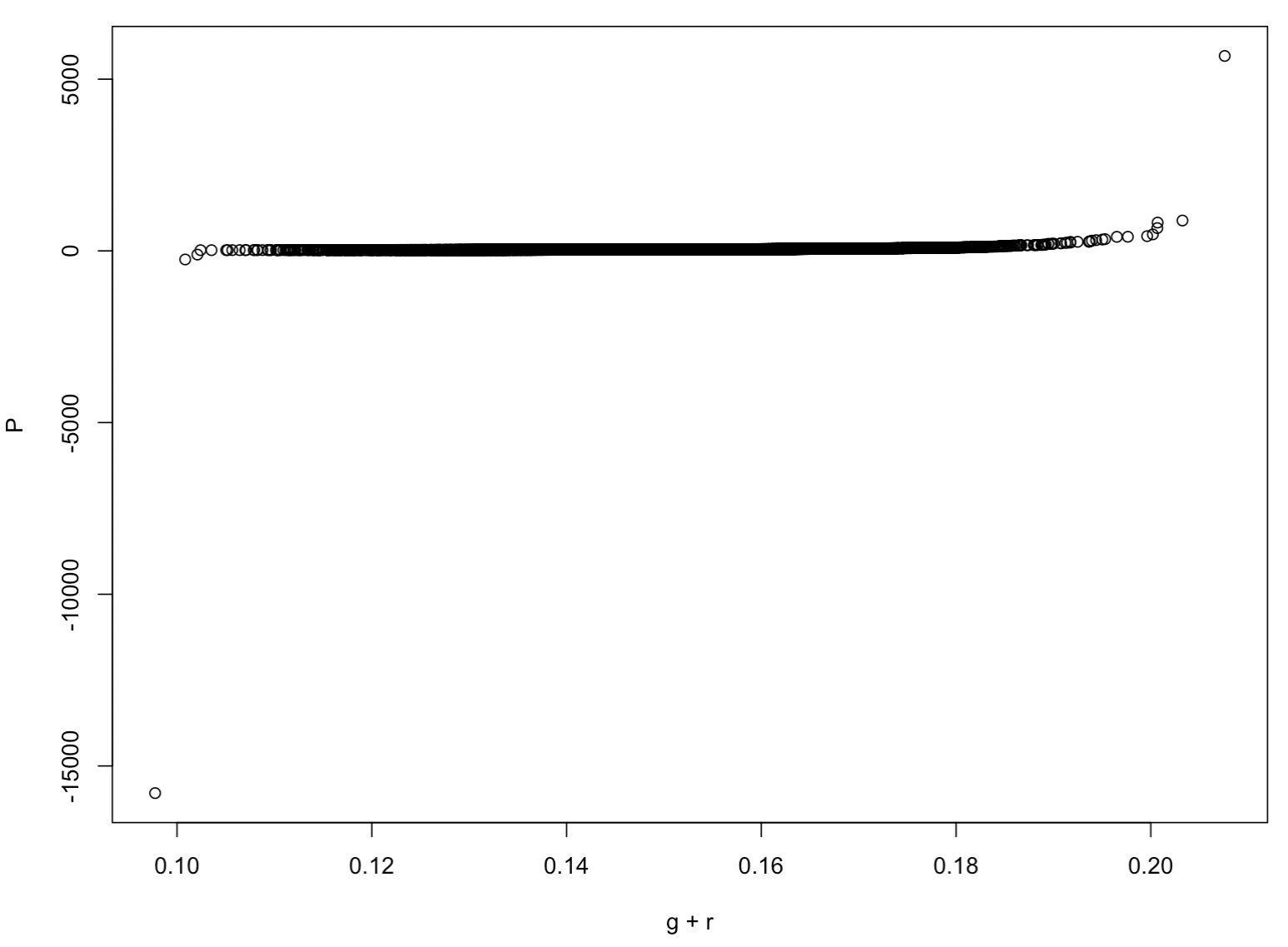
The low cost of equity/high growth rate firms do not pass, given their stock prices will be artificially inflated from the Gordon Growth Model framework, but all others perform reasonably well.

Conclusion

Linear regression does not work very well when estimating stock prices at low costs of equity and high growth rates when simulated from the context of the DDM model.

Nonetheless, if we are given a spreadsheet of company data within a particular economy, and broken down by sector, we could reasonably estimate stock prices from a linear regression model.

After all, stock prices at the most basic level trade at some expected multiple of annual earnings. If a sector is trading at 15x earnings and the company is mature and produces $5 of earnings per share, you might expect it to trade around $75.

If a linear regression takes into account this data, it should do a reasonable job of making this approximation.

We also wouldn’t be subject to the hypersensitivity of the factors of growth rate and cost of equity as we would under a DDM model.

However, financial modeling is naturally a spreadsheet-based undertaking and is naturally the way to value a stock’s price. Spreadsheets allow us to determine relationships by established financial formulas.

On the other hand, linear regression is inherently different by taking multiple rows of data and determining relationships by developing various multiple regression models.

From there we can observe what comes back as statistically significant and determine the appropriate magnitude of the coefficients to develop a predictive model like we’ve done on other forms of data.

While traditional spreadsheet applications are the standard approach to things in valuing companies, multiple linear regression provides another potential avenue to explore.